📚 Clustering
In a clustering task, we would like to divide the data into groups (called clusters) with similar properties (in some sense).
Two examples of cases in which we would like to cluster the data:
- We would like to uncover relationships in a dataset, in order to make deductions on the properties of a member based on the features of other members of his cluster. For example:
- Clustering customers in order to suggest a marketing strategy based on other members of a cluster. For example, we might try to advertise products which are popular among their cluster.
- Clustering plants and animals, given some known properties, in order to uncover some new properties they might have, based on the properties of the members of their cluster
- We would like to give a different treatment to each cluster based on its properties. As we will see in the example in this workshop.
There exist a variety of different clustering algorithms which take a different approach for clustering the data. Each algorithm leads to a different selection of clusters.
Examples of Different Clustering Algorithms
In the documentation of the scikit-learn package there is a comparison of the different clustering method implemented in the package on some 2D toy-models datasets:
https://scikit-learn.org/stable/auto_examples/cluster/plot_cluster_comparison.html
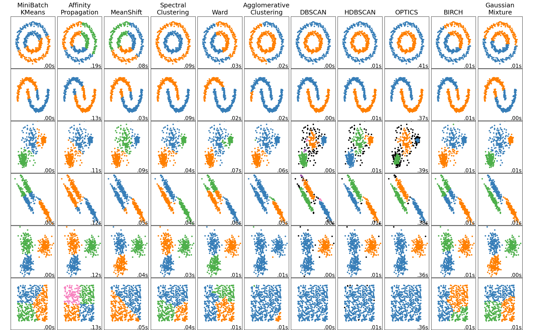
In this course, we will discuss the K-means algorithm.
K-Means
In K-means the number of clusters is selected a priori, and the objective of the algorithm is to divide the data into groups such that the sum of the averaged squared distances in each cluster is minimal.
I.e., by denoting as the -th cluster (), and as the number of points in the -th cluster, K-mean searches for the optimal clustering :
| it can easily be shown that this equivalent to minimizing the sum of squared distances from each point to the center the average point of its cluster $$\boldsymbol{\mu}_i=\frac{1}{\left | S_i\right | }\sum_{\boldsymbol{x}\in S_i}\boldsymbol{x}$$. I.e. |
To find the optimal clustering, K-mean works as follow:
Initialization
The algorithm is initialized by randomly selecting points, , which are to be used as an initial guess for the cluster’s centers.
A common initialization is to select point for the dataset.
Iterations
The algorithm then iteratively updates the clusters and the clusters’ centers by repeating these two steps:
-
Cluster the points by assign each point to the closest to it, while is kept fixed. The -th cluster is the set of points assigned to .
-
Updated the to be the new centers of each cluster, while keeping the assignments to clusters fixed.
These steps are repeated until the clusters reach a steady state (i.e., no updated in needed in the clustering stage)
It can be shown that this algorithm is guaranteed to converge to a minimum, but it is not guaranteed to converge to the global minimum.
Workshop 4
K-Means
🚖 The NYC Taxi Dataset
We will use the same dataset from the last two workshops. This time focusing on the drop off locations.
❓️ Problem: Finding The Optimal Parking Lots Locations
A taxi company is looking to rent parking lots so that their taxis can wait in them in between rides.
It would like to select the optimal locations to place these parking lots such that the average distance from the drop off location to the nearest parking lot will be minimal.
🔃 The workflow
We will follow the workflow which we have described in the previous workshops.

🛠️ Preparations
As usual, we will start by importing some useful packages
# Importing packages
import numpy as np  # Numerical package (mainly multi-dimensional arrays and linear algebra)
import pandas as pd  # A package for working with data frames
import matplotlib.pyplot as plt  # A plotting package
import skimage.io  # A package for working with images. A friendlier version of OpenCV but with less features. Specifically, here we import the io module for saving and loading images.


## Setup matplotlib to output figures into the notebook
## - To make the figures interactive (zoomable, tooltip, etc.) use ""%matplotlib notebook" instead
%matplotlib inline

plt.rcParams['figure.figsize'] = (5.0, 5.0)  # Set default plot's sizes
plt.rcParams['figure.dpi'] = 90  # Set default plot's dpi (increase fonts' size)
plt.rcParams['axes.grid'] = True  # Show grid by default in figures

## A function to add Latex (equations) to output which works also in Google Colabrtroy
## In a regular notebook this could simply be replaced with "display(Markdown(x))"
from IPython.display import HTML
def print_math(x):  # Define a function to preview markdown outputs as HTML using mathjax
    display(HTML(''.join(['<p><script src=\'https://cdnjs.cloudflare.com/ajax/libs/mathjax/2.7.3/latest.js?config=TeX-AMS_CHTML\'></script>',x,'</p>'])))
🕵️ Data Inspection (Reminder)
Print out the size and the 10 first rows of the dataset.
data_file = 'https://technion046195.github.io/semester_2019_spring/datasets/nyc_taxi_rides.csv'

## Loading the data
dataset = pd.read_csv(data_file)

## Print the number of rows in the data set
number_of_rows = len(dataset)
print_math('Number of rows in the dataset: $$N={}$$'.format(number_of_rows))

## Show the first 10 rows
dataset.head(10)
Number of rows in the dataset:
| passenger_count | trip_distance | payment_type | fare_amount | tip_amount | pickup_easting | pickup_northing | dropoff_easting | dropoff_northing | duration | day_of_week | day_of_month | time_of_day | |
|---|---|---|---|---|---|---|---|---|---|---|---|---|---|
| 0 | 2 | 2.768065 | 2 | 9.5 | 0.00 | 586.996941 | 4512.979705 | 588.155118 | 4515.180889 | 11.516667 | 3 | 13 | 12.801944 |
| 1 | 1 | 3.218680 | 2 | 10.0 | 0.00 | 587.151523 | 4512.923924 | 584.850489 | 4512.632082 | 12.666667 | 6 | 16 | 20.961389 |
| 2 | 1 | 2.574944 | 1 | 7.0 | 2.49 | 587.005357 | 4513.359700 | 585.434188 | 4513.174964 | 5.516667 | 0 | 31 | 20.412778 |
| 3 | 1 | 0.965604 | 1 | 7.5 | 1.65 | 586.648975 | 4511.729212 | 586.671530 | 4512.554065 | 9.883333 | 1 | 25 | 13.031389 |
| 4 | 1 | 2.462290 | 1 | 7.5 | 1.66 | 586.967178 | 4511.894301 | 585.262474 | 4511.755477 | 8.683333 | 2 | 5 | 7.703333 |
| 5 | 5 | 1.561060 | 1 | 7.5 | 2.20 | 585.926415 | 4512.880385 | 585.168973 | 4511.540103 | 9.433333 | 3 | 20 | 20.667222 |
| 6 | 1 | 2.574944 | 1 | 8.0 | 1.00 | 586.731409 | 4515.084445 | 588.710175 | 4514.209184 | 7.950000 | 5 | 8 | 23.841944 |
| 7 | 1 | 0.804670 | 2 | 5.0 | 0.00 | 585.344614 | 4509.712541 | 585.843967 | 4509.545089 | 4.950000 | 5 | 29 | 15.831389 |
| 8 | 1 | 3.653202 | 1 | 10.0 | 1.10 | 585.422062 | 4509.477536 | 583.671081 | 4507.735573 | 11.066667 | 5 | 8 | 2.098333 |
| 9 | 6 | 1.625433 | 1 | 5.5 | 1.36 | 587.875433 | 4514.931073 | 587.701248 | 4513.709691 | 4.216667 | 3 | 13 | 21.783056 |
The Data Fields and Types
This time we will be looking at the following two columns:
- dropoff_easting - The horizontal coordinate (east-west) in UTM-WGS84 (~ in kilometers)
- dropoff_northing - The vertical coordinate (north-south) in UTM-WGS84 (~ in kilometers)
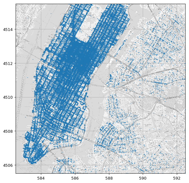
Plotting Drop Off Points
Just for having a nice visualization we will plot the points over the NYC map which can be found here
(the bounding box of the map image is: [582.5, 592.5, 4505.5, 4515.5] as [West East South North] coordinates in UTM-WSG84)
## Load and image of the streets of NY
ny_map_image = skimage.io.imread('../media/nyc_map.png')

## The geografic bounding box of the map data as [West-longtitude East-longtitude South-latitude North-latitude]:
bbox = [582.5, 592.5, 4505.5, 4515.5]
## Create the figure and axis
fig = plt.figure(figsize=(8, 8))
ax = fig.add_subplot(1, 1, 1)
ax.grid(True)

## Plot the map
ax.imshow(ny_map_image, extent=bbox, cmap='gray', alpha=0.7)
ax.plot(dataset['dropoff_easting'], dataset['dropoff_northing'], '.', markersize=1);
📜 Problem Definition
The underlying process
A random phenomenon generating taxi rides along with there details
The task and goal
Finding locations for parking lots such that the average distance to the nearest parking lot will be minimal.
Evaluation method
As stated in the goal, the quantity which we would like to minimize is given by:
- as the random variable of the drop off location.
- : as the location of the -th parking lot.
- : The number of points in the dataset.
We would like to define and minimize the following risk function:
Therefore, this will be our risk function.
As usual, since we do not know the exact distribution of so we would approximate the risk function with an empirical risk. In this case, we will replace the expectation value with the empirical mean calculated on a test set :
In fact, we can write this problem as a clustering problem. We can do so by rewriting the above summation as a summation over clusters where each cluster is defined by the location of the nearest parking lot.
By denoting the cluster of points for which is their closet parking lot as , we can rewrite the summation as:
📚 Splitting the Data
Let us split the data into 80% train set and 20% test set
n_samples = len(dataset)

## Generate a random generator with a fixed seed (this is important to make our result reproducible)
rand_gen = np.random.RandomState(0)

## Generating a vector of indices
indices = np.arange(n_samples)

## Shuffle the indices
rand_gen.shuffle(indices)

## Split the indices into 80% train / 20% test
n_samples_train = int(n_samples * 0.8)
train_indices = indices[:n_samples_train]
test_indices = indices[n_samples_train:]

train_set = dataset.iloc[train_indices]
test_set = dataset.iloc[test_indices]
💡 Model & Learning Method Suggestion
Model
In this case the model is in fact all possible solutions which is any set of 2D points.
Learning Method: K-Means
To solve this problem, we will use K-means. Note that K-means does not actually solve our exact problem since it minimizes the average squared Euclidean distance and not the average Euclidean distance itself. There are some more complicated algorithms for solving our exact problem, but for now we will stick to K-means.
This is, in fact, a common case where we do not have an efficient way to solve our exact so we solve a very similar problem with the understanding that the result which we will get will probably not be the optimal solution, but we hope that it will at least produce a satisfactory result.
⚙️ Learning
✍️ Exercise 4.1 - K-Means
- Use the data and k-means to select the location of 10 parking lots
- Evaluate the empirical risk on the train set
Solution 4.1-1
Lets us implement the K-means algorithm.
from scipy.spatial import distance # A function for efficiently calculating all the distances between points in two lists of points.
## Set K
k = 10
## Define x (the matrix of the drop off locations)
x = train_set[['dropoff_easting', 'dropoff_northing']].values
n_samples = len(x)
## Create a random generator using a fixed seed (we fix the seed for reproducible results)
rand_gen = np.random.RandomState(0)
## Initialize the means using k random points from the dataset
means = x[rand_gen.randint(low=0, high=n_samples, size=k)]
assignment = np.zeros(n_samples, dtype=int)
## Prepare figure and plotting counters
next_axis = 0
fig, axis_list = plt.subplots(3, 3, figsize=(12, 12))
i_step = 0
next_plot_step = 1
stop_iterations = False
while not stop_iterations:
i_step += 1
assignment_old = assignment
## Step 1: Assign points to means
distances = distance.cdist(x, means, 'euclidean')
assignment = np.argmin(distances, axis=1)
## Stop criteria
if (assignment == assignment_old).all():
stop_iterations = True
## Step 2: Update means
for i_cluster in range(k):
cluster_indices = assignment == i_cluster
means[i_cluster] = x[cluster_indices].mean(axis=0)
## Plot clusters and means
if (i_step == next_plot_step) or (stop_iterations):
ax = axis_list.flat[next_axis]
ax.grid(True)
ax.set_title('Step: {}'.format(i_step))
ax.imshow(ny_map_image, extent=bbox, cmap='gray', alpha=0.7)
for i_cluster in range(k):
cluster_indices = assignment == i_cluster
ax.plot(x[cluster_indices, 0], x[cluster_indices, 1], '.', markersize=1)
ax.plot(means[:, 0], means[:, 1], 'xk', markersize=20)[0]
next_plot_step *= 2
next_axis += 1
for i in range(next_axis, len(axis_list.flat)):
axis_list.flat[i].set_visible(False)
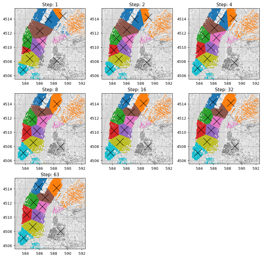
print('Number of steps: {}'.format(i_step))
parking_lots_locations = means
Number of steps: 63
From here on we will use the sklearn.cluster.KMeans class to run the K-means algorithm.
Solution 4.1-2
Let us evaluate the empirical risk function on the train set:
## Calculate distances to all parking lots
distances = distance.cdist(x, parking_lots_locations, 'euclidean')

## Calculate the average of the distances to the colsest parking lot to each point
train_risk = distances.min(axis=1).mean()

print('The average ride distance to the closest parking lots is approximately {:.02f} km'.format(train_risk))
The average ride distance to the closest parking lots is approximately 0.70 km
⏱️ Performance Evaluation
✍️ Exercise 4.2
- Evaluate the performance using parking lots locations which were selected using the K-means algorithms.
- Name 2 reasons why this solution is probably not the optimal solution.
- Suggest methods to improve our result based on each of the problems from the previous section.
Solution 4.2-1
Let us evaluate the empirical risk function on the test set:
## Define x for the test set
x_test = test_set[['dropoff_easting', 'dropoff_northing']].values

## Calculate distances to all parking lots
distances = distance.cdist(x_test, parking_lots_locations, 'euclidean')

## Calculate the average of the distances to the colsest parking lot to each point
test_risk = distances.min(axis=1).mean()

print('The average ride distance to the closest parking lots is approximatley {:.02f} km'.format(test_risk))
The average ride distance to the closest parking lots is approximatley 0.70 km
Solution 4.2-(2 & 3)
Two reasons, which we have already mentioned, for why K-means does not converge to the optimal parking lots selection:
-
K-means is only guaranteed to converge to a local minimum and not necessarily the global minimum. One way to slightly overcome this problem is to run the K-means algorithm several times using a different initialization each time.
-
K-means finds the optimal solution for minimizing the average squared distance. To improve our results, we can use the clusters selected by K-mean, but instead of using the mean point of the cluster, we can find the point which minimizes the sum of distances in each cluster.
A side note: The point which minimizes the sum of Euclidean distances is called The Geometric Median (wiki), and it can be found for example using an algorithm called the Weiszfeld’s algorithm.
❓️ Problem 2: Finding The Optimal Number of Parking Lots
Now let us address the topic of selecting the number of parking lots (the number of clusters)
Basically, to reduce the average ride distance we would like as much parking lots as possible, but in practice operating a parking lots cost money. Let us assume that:
- The price of operating a parking lot is 10k$ per month.
- There will be exactly 100k rides to the parking lots per month.
- The estimated price per kilometer for when driving to the parking is estimated at 3$ / kilometer.
📜 Problem Definition
✍️ Exercise 4.3
Following these assumptions write a risk function which is the expected mean total cost of driving to and operating the parking lots.
Solution 4.3
The risk function would be:
The empirical risk function would be:
💡 Model & Learning Method Suggestion
Now the space of solutions is the space of all possible locations and number of parking lots. We saw how to solve it for a fixed and we can easily run over all relevant values of to find the optimal value.
This is a common case in machine learning, where we have a method for fining an optimal model configuration only after we fix some parameters of the model. We will refer to this part of the model for which we do not have an efficient way to optimally select as the hyper-parameters of the model.
Two more hyper-parameters which we have encountered so far are:
- The number of bins in a histogram.
- The kernel and width in KDE.
Two approaches for selecting the hyper-parameters values are:
Brute Force / Grid Search
Some times, like in this case, we will be able to simply the relevant range of possible values of the hyper-parameters. In this case, our solution would be to simply loop over the relevant values and pick the ones which result in the minimal risk.
Trial and error
In other cases we would usually start by fixing these hyper-parameters manually according to some rule of thumb or some smart guess, and iteratively:
- Solve the model given the fixed hyper-parameters.
- Update the hyper-parameters according to the results we get.
The workflow revisited - Hyper-parameters
Let us add the loop/iterations over the hyper-parameters to our workflow

⚙️ Learning
✍️ Exercise 4.4
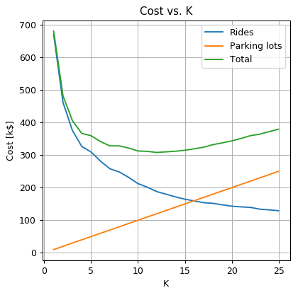
Use K-means to select the number and locations of parking lots. Search over the range of . Plot the empirical train risk as a function of .
Solution 4.4
## import KMeans from scikit-learn
from sklearn.cluster import KMeans
cost_per_parking = 10
cost_per_avarage_distance = 300
## Define the grid of K's over we will search for our solution
k_grid = np.arange(1, 26, 1)
## Initialize the list of the average ride distance
average_distance_array = np.zeros(len(k_grid), dtype=float)
## Create a random generator using a fixed seed
rand_gen = np.random.RandomState(0)
best_risk_so_far = np.inf
optimal_k = None
optimal_average_distance = None
optimal_centers = None
for i_k, k in enumerate(k_grid):
## Calculate ceneters and clusters
kmeans = KMeans(n_clusters=k, random_state=rand_gen)
assignments = kmeans.fit_predict(x)
centers = kmeans.cluster_centers_
## Evaluate the empirical risk
distances = np.linalg.norm(x - centers[assignments], axis=1)
average_distance = distances.mean()
risk = cost_per_parking * k + cost_per_avarage_distance * average_distance
## If this is the best risk so far save the optimal results
if risk < best_risk_so_far:
best_risk_so_far = risk
optimal_k = k
optimal_average_distance = average_distance
optimal_centers = centers
## Save average distance for the later plot
average_distance_array[i_k] = average_distance
print('The optimal number of parking lots is: {}'.format(optimal_k))
print('The optimal average ride distance is: {:.2f} Km'.format(optimal_average_distance))
print('The train risk is {:.02f} k$'.format(best_risk_so_far))
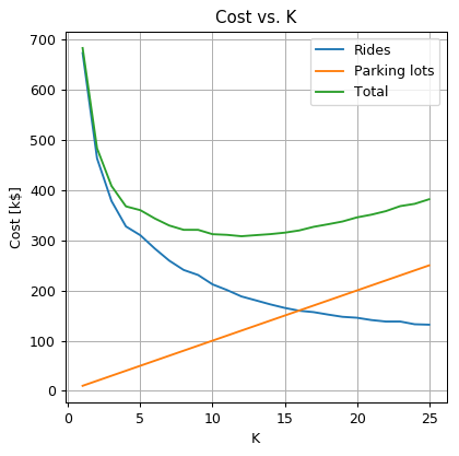
## Plot
fig, ax = plt.subplots()
ax.plot(k_grid, average_distance_array * cost_per_avarage_distance, label='Rides')
ax.plot(k_grid, k_grid * cost_per_parking, label='Parking lots')
ax.plot(k_grid, k_grid * cost_per_parking + average_distance_array * cost_per_avarage_distance, label='Total')
ax.set_title('Cost vs. K')
ax.set_ylabel('Cost [k$]')
ax.set_xlabel('K')
ax.legend();
The optimal number of parking lots is: 12
The optimal average ride distance is: 0.63 Km
The train risk is 308.12 k$
⏱️ Performance evaluation
## Calculate distances to all parking lots
distances = distance.cdist(x_test, optimal_centers, 'euclidean')

## Calculate the average distance and risk
test_average_distance = distances.min(axis=1).mean()
test_risk = cost_per_parking * optimal_k + cost_per_avarage_distance * test_average_distance

print('The optimal average ride distance is: {:.2f} Km'.format(test_average_distance))
print('The train risk is {:.2f} k$'.format(test_risk))
The optimal average ride distance is: 0.63 Km
The train risk is 307.81 k$
Train-Validation-Test Separation
In the above example, we have selected the optimal based upon the risk which was calculated using the train set. As we stated before this situation is problematic since the risk over the test set would be too optimistic due to overfitting. This is mainly problematic, but not limited to, the case where we have a small amount of data. For example, think about the extreme case where there were only 5 data points. In this case, the training risk will obviously be lower than the true risk and would even go down to zero for .
The solution to this problem is to also divide the dataset once more. Therefore in cases, where we would also be required to optimize over some hyper-parameters, we would divide our data into three sets: a train-set a validation-set and a test-set.
A common practice is to use 60% train - 20% validation - 20% test.
✍️ Exercise 4.5
Repeat the learning process using the 3-fold split. Did the results change significantly? Why?
Solution 4.5
We shall start by splitting the data
## Generate a random generator with a fixed seed
rand_gen = np.random.RandomState(0)

## Generating a vector of indices
indices = np.arange(n_samples)

## Shuffle the indices
rand_gen.shuffle(indices)

## Split the indices into 80% train / 20% test
n_samples_train = int(n_samples * 0.6)
n_samples_validation = int(n_samples * 0.2)
n_samples_test = n_samples - n_samples_train
train_indices = indices[:n_samples_train]
validation_indices = indices[n_samples_train:(n_samples_train + n_samples_validation)]
test_indices = indices[(n_samples_train + n_samples_validation):]

train_set = dataset.iloc[train_indices]
validation_set = dataset.iloc[validation_indices]
test_set = dataset.iloc[test_indices]
Now we can repeat the learning stage
## Updates the datasets
x = train_set[['dropoff_easting', 'dropoff_northing']].values
x_validation = validation_set[['dropoff_easting', 'dropoff_northing']].values
x_test = test_set[['dropoff_easting', 'dropoff_northing']].values

## Initialize the list of the average ride distance
average_distance_array = np.zeros(len(k_grid), dtype=float)

## Create a random generator using a fixed seed
rand_gen = np.random.RandomState(0)

best_risk_so_far = np.inf
optimal_k = None
optimal_average_distance = None
optimal_centers = None
for i_k, k in enumerate(k_grid):

    ## Calculate ceneters and clusters
    kmeans = KMeans(n_clusters=k, random_state=rand_gen)
    kmeans.fit(x)
    centers = kmeans.cluster_centers_

    ## Evaluate the empirical risk
    assignments = kmeans.predict(x_validation)
    distances = np.linalg.norm(x_validation - centers[assignments], axis=1)
    average_distance = distances.mean()
    risk = cost_per_parking * k + cost_per_avarage_distance * average_distance

    ## If this is the best risk so far save the optimal results
    if risk < best_risk_so_far:
        best_risk_so_far = risk
        optimal_k = k
        optimal_average_distance = average_distance
        optimal_centers = centers

    ## Save average distance for the later plot
    average_distance_array[i_k] = average_distance

## Plot
fig, ax = plt.subplots()
ax.plot(k_grid, average_distance_array * cost_per_avarage_distance, label='Rides')
ax.plot(k_grid, k_grid * cost_per_parking, label='Parking lots')
ax.plot(k_grid, k_grid * cost_per_parking + average_distance_array * cost_per_avarage_distance, label='Total')
ax.set_title('Cost vs. K')
ax.set_ylabel('Cost [k$]')
ax.set_xlabel('K')
ax.legend();

## Calculate the test results
distances = distance.cdist(x_test, optimal_centers, 'euclidean')
test_average_distance = distances.min(axis=1).mean()
test_risk = cost_per_parking * optimal_k + cost_per_avarage_distance * test_average_distance

print('The optimal number of parking lots is: {}'.format(optimal_k))
print('The optimal average ride distance is: {:.2f} Km'.format(test_average_distance))
print('The train risk is {:.2f} k$'.format(test_risk))
The optimal number of parking lots is: 12
The optimal average ride distance is: 0.63 Km
The train risk is 308.04 k$
As the same as got without the validation-split, the optimal is 12. In this case, the amount of data is large, and the apparent overfit seems to be small. In general, it will usually be hard to tell if our dataset is large enough, and how much overfit do we have in our solution.
%%html
<link rel="stylesheet" href="../css/style.css"> <!--Setting styles - You can simply ignore this line-->