Hands-on

🚖 Reminder: The NYC Taxi Dataset

The first 10 out of 100k taxi rides in NYC.

	passenger_count	trip_distance	payment_type	fare_amount	tip_amount	pickup_easting	pickup_northing	dropoff_easting	dropoff_northing	duration	day_of_week	day_of_month	time_of_day
0	2	2.768065	2	9.5	0.00	586.996941	4512.979705	588.155118	4515.180889	11.516667	3	13	12.801944
1	1	3.218680	2	10.0	0.00	587.151523	4512.923924	584.850489	4512.632082	12.666667	6	16	20.961389
2	1	2.574944	1	7.0	2.49	587.005357	4513.359700	585.434188	4513.174964	5.516667	0	31	20.412778
3	1	0.965604	1	7.5	1.65	586.648975	4511.729212	586.671530	4512.554065	9.883333	1	25	13.031389
4	1	2.462290	1	7.5	1.66	586.967178	4511.894301	585.262474	4511.755477	8.683333	2	5	7.703333
5	5	1.561060	1	7.5	2.20	585.926415	4512.880385	585.168973	4511.540103	9.433333	3	20	20.667222
6	1	2.574944	1	8.0	1.00	586.731409	4515.084445	588.710175	4514.209184	7.950000	5	8	23.841944
7	1	0.804670	2	5.0	0.00	585.344614	4509.712541	585.843967	4509.545089	4.950000	5	29	15.831389
8	1	3.653202	1	10.0	1.10	585.422062	4509.477536	583.671081	4507.735573	11.066667	5	8	2.098333
9	6	1.625433	1	5.5	1.36	587.875433	4514.931073	587.701248	4513.709691	4.216667	3	13	21.783056

❓️ Same Problem: Estimating the Distribution of Trip Duration

We would like to estimate the distribution of the rides durations and represent them as a CDF or a PDF.

💡 Method I: Normal Distribution + MLE

• In this case we will try to use a normal distribution as our parametric model.
• The model parameters are its mean value $\mu$ and standard deviation $\sigma$.

Assumptions and notations:

• $N$ - The number of samples points in the dataset.
• $\boldsymbol{\theta}=\left[\mu,\sigma\right]^T$ - The vector of parameters.
• $p_\text{normal}\left(x_i;\boldsymbol{\theta}\right)=\frac{1}{\sqrt{2\pi\sigma^2}}\exp\left(-\frac{\left(x_i-\mu\right)^2}{2\sigma^2}\right), i=1,...,N$ - our model.

The negative log-likelihood function for the normal distribution model is then:

$$\begin{align*} -l_\text{normal}\left(\boldsymbol{\theta}\ ;\boldsymbol{x}\right) & = -\log\left(\mathcal{L}_\text{normal}\left(\boldsymbol{\theta}\right|\boldsymbol{x})\right) \\ & = -\log\left(\prod_i p_\text{normal}\left(x_i;\boldsymbol{\theta}\right)\right) \\ & = -\sum_i\log\left(p_\text{normal}\left(x_i;\boldsymbol{\theta}\right)\right) \\ & = -\sum_i\log\left(\frac{1}{\sqrt{2\pi\sigma^2}}\exp\left(-\frac{\left(x_i-\mu\right)^2}{2\sigma^2}\right)\right) \\ & = N\log\left(\sqrt{2\pi}\sigma\right)+\frac{1}{2\sigma^2}\sum_i\left(x_i-\mu\right)^2 \\ \end{align*}$$

Under the MLE approach, the optimal parameters $\boldsymbol{\theta}^*$ for the model are given by

$$\begin{align*} \hat{\boldsymbol{\theta}} & = \underset{\boldsymbol{\theta}}{\arg\min}\ -l_\text{normal}\left(\boldsymbol{\theta};\{x\}\right) \\ & = \underset{\boldsymbol{\theta}=\left(\mu,\sigma\right)^T}{\arg\min}\ N\log\left(\sqrt{2\pi}\sigma\right)+\frac{1}{2\sigma^2}\sum_i\left(x_i-\mu\right)^2 \\ \end{align*}$$

In the special case of MLE and a normal distribution, the optimization problem can be solved analytically. Sadly, this will not be true in the general case, and we will have to resort to numerical solutions.

We will find the solution for this optimization problem by comparing the derivative of the log-likelihood function to zero.

$$\begin{align*} & \begin{cases} \displaystyle{\frac{\partial l\left(\boldsymbol{\theta}|\boldsymbol{x}\right)}{\partial\mu}}=0 \\ \displaystyle{\frac{\partial l\left(\boldsymbol{\theta}|\boldsymbol{x}\right)}{\partial\sigma}}=0 \\ \end{cases} \\ \Leftrightarrow & \begin{cases} \displaystyle{\frac{\sum_i\left(x_i-\mu\right)}{\sigma^2}}=0 \\ \displaystyle{-\frac{N}{\sigma}+\frac{2\sum_i\left(x_i-\mu\right)^2}{2\sigma^3}}=0 \\ \end{cases}\\ \Leftrightarrow & \begin{cases} \mu=\displaystyle{\frac{1}{N}\sum_i x_i} \\ \sigma=\sqrt{\displaystyle{\frac{1}{N}\sum_i\left(x_i-\mu\right)^2}} \\ \end{cases} \end{align*}$$

Which results in our case in:

$$\hat{\mu} = 11.4\ \text{min}$$ $$\hat{\sigma} = 7.0\ \text{min}$$

We will plot the estimated PDF on top of the histogram.

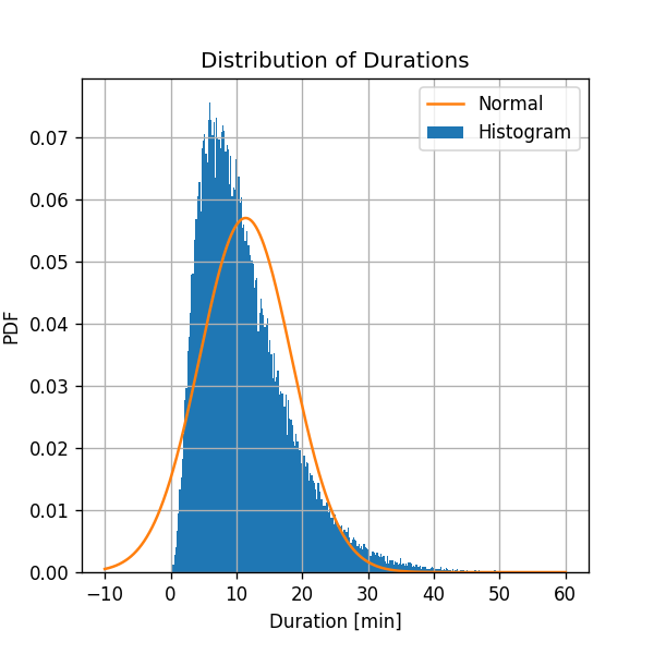
It seems that the normal distribution gives a very rough approximation of the real distribution. In some cases this would be good enough as a first order approximation, but in this case we would like to do better.

One very disturbing fact, for example, is that there is a non zero probability to get negative ride durations, which is obviously not realistic.

Let us try to propose a better model in order to get a better approximation.

💡 Method II : Rayleigh Distribution + MLE

The Rayleigh distribution describes the distribution of the magnitude of a 2D Gaussian vector with zero mean and no correlation between it’s two components. In other words, if $Z$ has the following distribution:

$$\boldsymbol{Z}\sim N\left(\begin{bmatrix} 0 \\ 0 \end{bmatrix}, \begin{bmatrix} \sigma^2 & 0 \\ 0 & \sigma^2 \end{bmatrix}\right)$$

Than $\left\lVert\boldsymbol{Z}\right\rVert_2=\sqrt{Z_x^2+Z_y^2}$ has a Rayleigh distribution.

The PDF of the Rayleigh distribution is given by:

$$p_\text{Rayleigh}\left(z;\sigma\right)=\frac{z}{\sigma^2}\exp\left({-\frac{z^2}{2\sigma^2}}\right), \quad z\geq0$$

Notice that here the distribution is only defined for positive values. The Rayleigh distribution has only one parameter $\sigma$ which is called the scale parameter. Unlike in case of the normal distribution, here $\sigma$ is not equal to the standard deviation.

For consistency we will denote the 1D vector of parameters: $\boldsymbol{\theta}=\left[\sigma\right]$

We will give a short motivation for preferring the Rayleigh distribution.

Motivation For Using Rayleigh Distribution

We have started with an assumption that the duration a taxi ride is normally distributed. Let us instead assume that the quantity which is normally distributed is the 2D distance $\boldsymbol{D}$, between the pickup location to the drop off location.

In other words, we are assuming that the random variable $\boldsymbol{D}$ is a 2D Gaussian vector. For simplicity, we will also assume that the $x$ and $y$ components of $\boldsymbol{D}$ are uncorrelated with equal variance and zero mean, i.e. we assume that: $\boldsymbol{D}\sim N\left(\begin{bmatrix} 0 \\ 0 \end{bmatrix}, \begin{bmatrix} \sigma_D^2 & 0 \\ 0 & \sigma_D^2 \end{bmatrix}\right)$ In addition, let us also assume that the taxis speed, $v$ is constant. Therefore the relation between the ride duration $T$ and the distance vector $\boldsymbol{D}$ is:

$$T = \frac{\left\lVert D\right\rVert_2}{v}$$

In this case $T$ will have a Rayleigh distribution with a scale parameter $\sigma=\frac{\sigma_D}{v}$.

The model in this case will be:

$$p_\text{rayleigh}\left(\boldsymbol{x};\boldsymbol{\theta}\right)=\prod_{i=1}^{N}\frac{x_i}{\sigma^2}\exp\left(-\frac{x_i^2}{2\sigma^2}\right)$$

The negative log-likelihood function will be:

$$\begin{align*} -l_\text{rayleigh}\left(\boldsymbol{\theta}|\{x\}\right) & = -\sum_i\log\left(p_\text{rayleigh}\left(x_i;\boldsymbol{\theta}\right)\right) \\ & = -\sum_i\log\left(x_i\right)+2N\log\left(\sigma\right)+\frac{1}{2\sigma^2}\sum_ix_i^2 \end{align*}$$

Our optimization problem will now be: $\hat{\boldsymbol{\theta}}=\underset{\boldsymbol{\theta}}{\arg\min}\ -\sum_i\log\left(x_i\right)+2N\log\left(\sigma\right)+\frac{1}{2\sigma^2}\sum_ix_i^2$ This optimization problem can be solved analytically. The solution will be:

$$\frac{\partial l_\text{rayleigh}\left(\theta|\{x\}\right)}{\partial\sigma}=0 \\ \Leftrightarrow -\frac{2N}{\sigma}+\frac{\sum_ix^2}{\sigma^3}=0 \\ \Leftrightarrow \sigma = \sqrt{\frac{1}{2N}\sum_i x^2}$$

Which results in:

$$\hat{\sigma} = 9.5$$

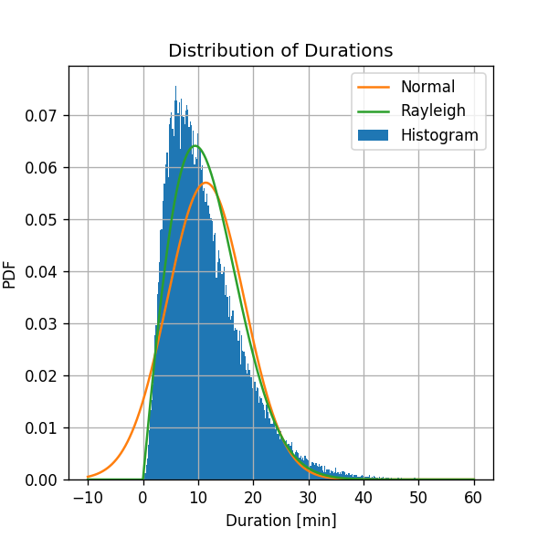
Judging by the similarity to the histogram, the Rayleigh distribution does a slightly better job at approximating the distribution and solves the negative values problem.

Let us try one more model.

💡 Method III: Generalized Gamma Distribution + MLE

The Rayleigh distribution is a special case of a more general family of distributions called the Generalized Gamma distribution. The PDF of the Generalized Gamma distribution is given by the following expression:

$$p_\text{gengamma}\left(z;\sigma,a,c\right)= \frac{cz^{ca-1}\exp\left(-\left(z/\sigma\right)^c\right)}{\sigma^{ca-1}\Gamma\left(a\right)} , \quad z\geq0$$

($\Gamma$ here is the gamma function)

This model has 3 parameters: $\boldsymbol{\theta}=\left[\sigma, a, c\right]^T$

For $c=2$ and $a=1$ we get the Rayleigh distribution (where $\sigma_{gamma}=2\sigma_{rayleigh}$ ).

Unlike the case of the normal and Rayleigh distributions, here we will not be able to find a simple analytic solution for the optimal MLE parameters. However we can use numerical methods for finding the optimal parameters. In practice we will use SciPy’s model for the General Gamma distribution to find the optimal parameters. You will use a similar method in your homework assignments.

By using SciPy’s numerical solver we get the following result:

$$\hat{a} = 4.4$$ $$\hat{c} = 0.8$$ $$\hat{\sigma} = 1.6$$

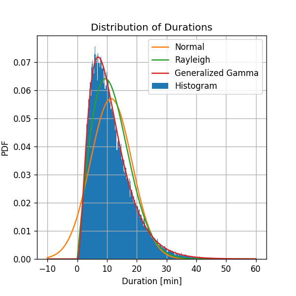
The Generalized Gamma distribution results in a distribution with a PDF which is much similar to the shape of the histogram.