Theory: Estimating Distributions

In the previous tutorial we have learned how to give a prediction for the case in which we know the distribution of some random variables, but in practice, in most cases we will not know the actual distribution of the random variables. In this tutorial we will see a few ways to estimate the distribution of random variables from a given set of measurements.

• We will call the set of data points the dataset.
• We will always assume here that the samples in the dataset are statistically independent.

Notations:

• $N$ - the number of samples in the dataset.
• $\omega_i$ - the $i$-th sample.
• $X$, $Y$ - Random variables.
• $D=\left\lbrace x_i\right\rbrace_{i=1}^N$ - The dataset ($N$ i.i.d samples of $X$)
• $x_i=X\left(\omega_i\right)$ - the realization related to $\omega_i$. Usually referred to as the data points.
• $p_X\left(x\right)$ - The PMF / PDF of a random variable.
• $F_X\left(x\right)$ - The CDF.

• $I\left\lbrace E\right\rbrace$ - An indicator function of whether condition $E$ is true. For example $I\left\lbrace x<y\right\rbrace=\begin{cases}1\ \text{if}\ x<y\\0\ \text{else}\end{cases}$.

• We will us the “hat” sign to denote an estimation of some unknown value. For example, we shall use $\hat{y}$ as our estimation for $y$.

Our goal in this tutorial is to estimate the distribution of $X$ by using the dataset.

🧮 Empirical Measure

The empirical measure, $\hat{p}_A$, is an estimation of the probability measure, $Pr\left(A\right)$, of some event $A$, given a set of samples.

$$\hat{p}_A=\tfrac{1}{N}\sum_{i=1}^N I\left\lbrace\omega_i\in A\right\rbrace$$

Put in words, we estimate the probability of an event as the fraction of samples in the dataset which are members of the event.

🎯 Empirical mean

The empirical mean, $\hat\mu_X$, is an estimation of the expectation value, $\mu_X=\mathbb{E}\left[X\right]$, of some random variable $X$

$$\hat{\mu}_X=\tfrac{1}{N}\sum_{i=1}^N x_i$$

We can of course replace $X$ with any function of $X$:

$$\hat{\mu}_{f\left(x\right)}=\tfrac{1}{N}\sum_{i=1}^N f\left(x_i\right)$$

📊 Estimating the PMF (Probability Mass Function)

(PDF in the discrete case)

We can estimate the PMF of a random variable using the empirical measure for each possible values of $X$.

$$\hat{p}_{X}\left(x\right)=\tfrac{1}{N}\sum_{i=1}^N I\left\lbrace x_i = x\right\rbrace$$

📈 Estimating the CDF (Cumulative Distribution Function)

Also known as ECDF (Empirical Cumulative Distribution Function).

Again, we can estimate the CDF using the empirical measure:

$$\hat{F}_{X}\left(x\right)=\tfrac{1}{N}\sum_{i=1}^N I\left\lbrace x_i \leq x\right\rbrace$$

Comment: The ECDF results in a non-continuous CDF which is a sum of step functions.

📶 Estimating the PDF using an Histogram

A histogram is a method of estimating the PDF (probability density function).

The idea is as follows:

• “Quantize” $X$ into a discrete set of values by dividing the range of values $X$ to a set of non-overlapping bins.
• Estimate the probability of being in bin - which is a task of estimating a PMF.
• Use a uniform distribution for the distribution of values inside each bin.

Notation:

• $l_k$, $r_k$ - The left and right edges of the $k$’s bin.

$$h_X\left(l_k \leq x < r_k\right) = \underbrace{\tfrac{1}{N}\sum_{i=1}^N I\left\lbrace l_k \leq x_i < r_k\right\rbrace}_\text{The probability of being in the k-th bin}\cdot\underbrace{\tfrac{1}{r_k-l_k}}_\text{Uniform distribution inside the bin}$$

Comment: The selection of the bins significantly effects how well the histogram approximates the PDF.

A common rule of thumb for selecting the bins is to divide the range of values into $\sqrt{N}$ equal bins.

📉 Estimating the PDF using Kernel Density Estimation (KDE)

KDE is another method for estimating the PDF. In KDE in KDE we produce a smooth distribution using a smoothing function called the Parzan window or the KDE kernel.

Two common choices of the Parzen window/kernal are:

• A Gaussian: $\phi\left(x\right)=\frac{1}{\sqrt{2\pi}}\exp\left(-\frac{x^2}{2}\right)$
• A rectangular function: $\phi\left(x\right)=I\left\lbrace\left\lvert x\right\rvert\leq0.5\right\rbrace$

A valid Parzen window will always be a valid PDF (positive and with an integral equal to 1)

One way to construct this smoothed distribution is:

• Start with a distribution which consists of $N$ delta functions of hight $\tfrac{1}{N}$ at the position of each sample.
• Smooth out the distribution by convolving it with the Parzen window.

The resulting distribution is given by:

$$\hat{p}_{\phi,X}\left(x\right) = \frac{1}{N}\sum_{i=1}^N \phi\left(x-x_i\right)$$

It is common to add a scaling factor $\alpha$, called the bandwidth, to control the width of the Parzen window. We shall denote the scaled version of the window by $\phi_h\left(x\right)=\frac{1}{\alpha}\phi\left(\frac{x}{\alpha}\right)$. Plugging this into the definition of the KDE, we get:

$$\hat{p}_{\phi,\alpha,X}\left(x\right) = \frac{1}{N\cdot\alpha}\sum_{i=1}^N \phi\left(\frac{x-x_i}{\alpha}\right)$$

For the two kernels above, this results in:

• A rectangular function: $\phi_{\alpha}\left(x\right)=\frac{1}{\alpha}I\left\lbrace\left\lvert x\right\rvert\leq0.5\alpha\right\rbrace$

• A Gaussian: in this case $a$ will in fact be the standard deviation of the Gaussian, so we will use $\sigma$ instead of $\alpha$ here: $\phi_{\sigma}\left(x\right)=\frac{1}{\sqrt{2\pi}\sigma}\exp\left(-\frac{x^2}{2\sigma^2}\right)$

A rule of thumb for selecting the bandwidth for the Gaussian window is: $\sigma=\left(\frac{4\cdot\text{std}\left\lbrace x_i\right\rbrace}{3N}\right)^\frac{1}{5}$

Estimations as Random Variables

It is important to notice here that each of the above estimations is in fact a random variable, since it is a function of the dataset, which is a collection of random variables. A single sample is this case is the entire set of $N$ data points which produces a single estimation.

We can think of repeating the process of generating $N$ data points over and over again, producing different estimations, and looking at the distribution of these estimations.

Let us denote by $\Theta$ the quantity which we would like to estimate, for example a probability measure, the ECDF of some value, etc. We can look for example at the mean of the estimation:

$$\mu_{\hat\theta}=\mathbb{E}\left[\hat{\theta}\left(D\right)\right]$$

Bias

The Bias of an estimation $\hat{\theta}\left(D\right)$ is the mean estimation error and is defined as:

$$\text{Bias}\left(\hat{\theta}\left(D\right)\right)\triangleq\mathbb{E}\left[\hat{\theta}\left(D\right)\right]-\theta=\mu_{\hat\theta}-\theta$$

(When the bias of an estimator is zero, we say the the estimator is unbiased)

Estimator Variance

Like every random variable, the Variance of an estimation is equal to:

$$\text{Var}\left(\hat{\theta}\left(D\right)\right)=\mathbb{E}\left[\left(\hat{\theta}\left(D\right)-\mu_{\hat\theta}\right)^2\right]=\mathbb{E}\left[\hat{\theta}^2\left(D\right)\right]-\mu_{\hat\theta}^2$$

The variance of and estimation describes the spread of the estimations. For a small variance, the estimations will be concentrated around the mean, while for a large variance the estimations will be spread out. In general, we would like the variance of our estimation to be small.

Hands-on

🚖 The NYC Taxi Dataset

As part of the effort of NYC to make its data publicly available and accessible, the city releases every month the full list of all taxi rides around the city. We will be using the dataset from January 2016, which can be found here

The full dataset includes over 10M taxi rides. In our course, we will be using a smaller subset of this dataset with only 100k rides (which has also been cleaned up a bit). The smaller dataset can be found here

The Data Fields and Types

Here are the first 10 rows in the dataset:

	passenger count	trip distance	payment type	fare amount	tip amount	pickup easting	pickup northing	dropoff easting	dropoff northing	duration	day of week	day of month	time of day
0	2	2.768065	2	9.5	0.00	586.996941	4512.979705	588.155118	4515.180889	11.516667	3	13	12.801944
1	1	3.218680	2	10.0	0.00	587.151523	4512.923924	584.850489	4512.632082	12.666667	6	16	20.961389
2	1	2.574944	1	7.0	2.49	587.005357	4513.359700	585.434188	4513.174964	5.516667	0	31	20.412778
3	1	0.965604	1	7.5	1.65	586.648975	4511.729212	586.671530	4512.554065	9.883333	1	25	13.031389
4	1	2.462290	1	7.5	1.66	586.967178	4511.894301	585.262474	4511.755477	8.683333	2	5	7.703333
5	5	1.561060	1	7.5	2.20	585.926415	4512.880385	585.168973	4511.540103	9.433333	3	20	20.667222
6	1	2.574944	1	8.0	1.00	586.731409	4515.084445	588.710175	4514.209184	7.950000	5	8	23.841944
7	1	0.804670	2	5.0	0.00	585.344614	4509.712541	585.843967	4509.545089	4.950000	5	29	15.831389
8	1	3.653202	1	10.0	1.10	585.422062	4509.477536	583.671081	4507.735573	11.066667	5	8	2.098333
9	6	1.625433	1	5.5	1.36	587.875433	4514.931073	587.701248	4513.709691	4.216667	3	13	21.783056

In this exercise we will only be interested in the two following columns:

• duration: The total duration of the ride (in minutes)
• time_of_day: A number between 0 and 24 indicating the time of the pickup. The integer part is the hour in 24H format and the decimal part are the minutes and seconds

(A full description for each of the other columns can be found here)

❓️ Problem: Estimating the Distribution of Trip Duration

A taxi driver would like to give an estimation for the distributions of trip durations. He has taken the course in machine learning and has figured that he can use historical rides data to estimate this distribution. Let us help the driver with his estimation.

Formally, we would like to estimate the distribution of the rides durations and represent them as a CDF or a PDF.

💡 Method I: ECDF

• We shall denote the set of 100k ride durations as $\left\lbrace x_i\right\rbrace$
• We shall calculate the ECDF numerically over a grid with a step size 0.001 min from $0$ to $\max\left(\left\lbrace x_i\right\rbrace\right)$

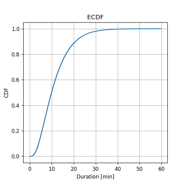
Note that the ECDF is a sum of step functions.

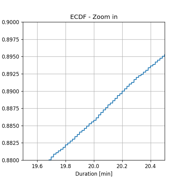
✍️ Question

According to the ECDF graph, what is the estimated probability of a ride to have a duration longer than 20 min?

Solution

The CDF graph describes the probability of $X_\text{duration}\leq x$. We want to evaluate:

$$P\left(X_\text{duration}>20 \text{min}\right)=1 - P\left(X_\text{duration}\leq 20 \text{min}\right)=1-\hat{F}_{X}\left(20\right)=1-0.89=0.11$$

The Dependency on the Dataset’s size

To see the dependency of the ECDF on the dataset’s size we shall recalculate the EDCF using a smaller amount of data. We will randomly sample N = 10, 100 and 1000 samples from the train set and use them to calculate the ECDF.

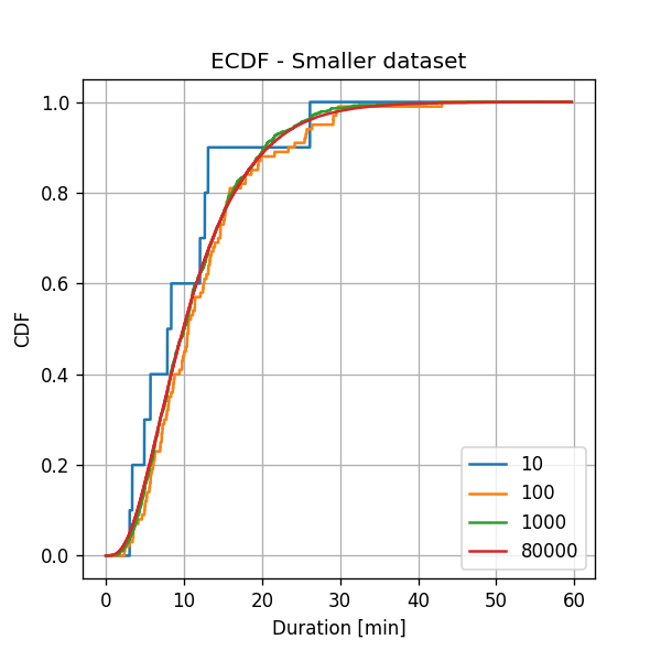
Not surprisingly, we can see that as we increase the number of points, the estimation becomes smoother, and although we have not defined an evaluation method, we will note that for all the popular distribution evaluation methods the error indeed decreases.

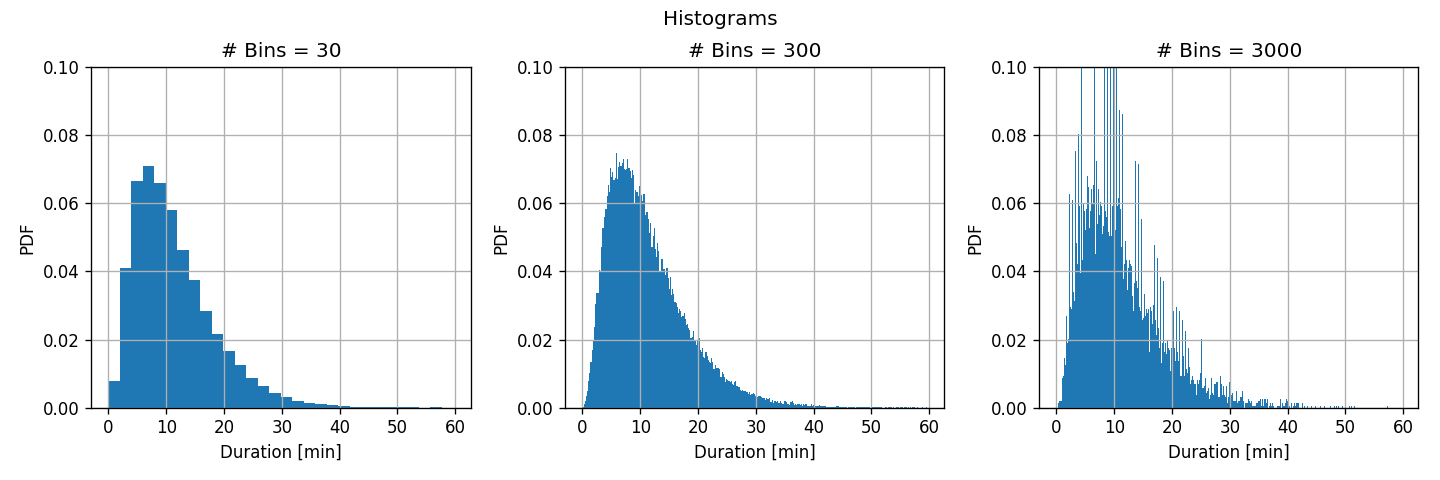
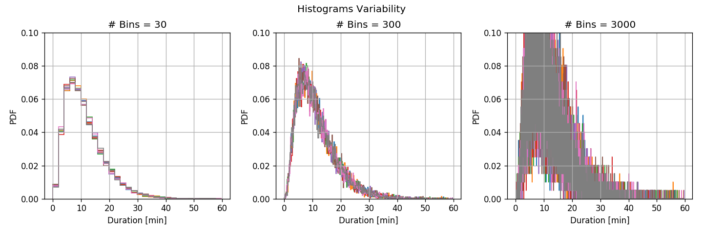
💡 Method II: Histogram

We shall calculate the histogram of ride durations using 30, 300 and 3000 bins.

Reminder: the rule of thumb suggests to use a number of bins equal to $\sqrt{N}=\sqrt{80000}\approx 280$

Before we examine the results we shall run another test. We shall split the train set into 8 equal subsets and calculate the histogram for each of the subsets.

To better visualize the variance let us plot the above graphs after removing the mean value:

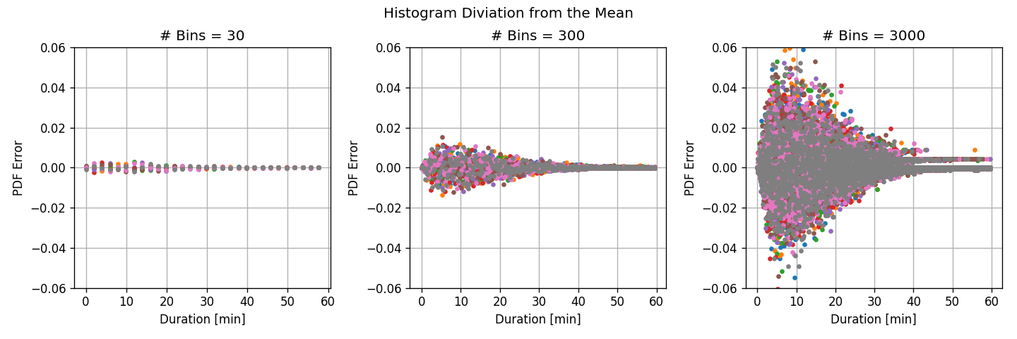
• For a large number of bins, the deviations between the subsets are large, but the bins are narrow.
  • high variance - large deviations between different subsets
  • low bias - small discretization error.
• For the small number of bins, the deviations between the subsets are small, but the bins are wide.
  • low variance - small deviations between different subsets.
  • high bias - large discretization error (the histogram is less smooth)

The Sources of Error

• Using a large amount of bins, the main source of error is due to the stochastic nature of the process which results in a high variance in our estimation. This error will be very significant for a small amount of data, but it will decrease as we add more data.
• Using a small number of bins, the main source of estimation error will be mostly due to the model’s limited representation capability (high bias). This type of error is unrelated to the amount of data.
• We should minimize the bias-variance tradeoff by setting the number of bins to an intermediate value. In this sense, the middle graphs gives the best results. Notice that it is close to the value predicted by the rule of thumb.

💡 Method III: KDE

We shall estimate the PDF of ride durations using KDE using a Gaussian Parzen window with bandwidth ($\sigma$) of 0.08, 0.8, 8.

Reminder: the rule of thumb suggests a width of: $\sigma=\left(\frac{4\cdot\text{std}\left\lbrace x_i\right\rbrace}{3N}\right)^\frac{1}{5}\approx0.775$

We will plot the resulting PDFs on top of the histogram with 300 bins for comparison.

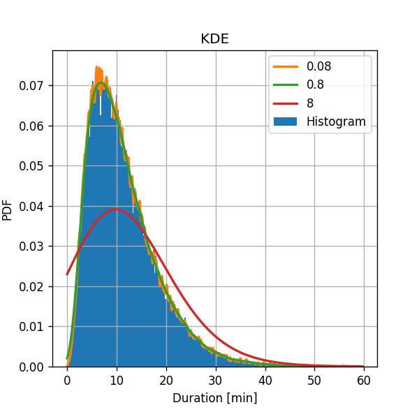
Again we see behavior similar to that of the histogram:

• For a narrow bandwidth, we get finer details, but the estimation is more “noisy”.

  • low bias
  • high variance of the estimation.

• For a wide bandwidth, we get fewer details, but we expect the estimation to have smaller variance.

  • high bias
  • low variance

❓️ Problem: Work Hours Prediction

We would like to predict whether a random given ride has occurred during the work hours or not, based only on the duration of the ride.

We shall define the work hours as between 7 a.m. and 18 p.m.

Let define the random binary variable $Y$:

$Y$ is equal to 1 if a ride occurred during the work hours, and 0 otherwise.

We shall denote the PMF of $Y$ by $p_Y\left(y\right)$

We will use the misclassification rate as a risk function:

​ $R(\hat y) = \frac{1}{N} \sum_{i=0}^N I\{\hat y(x_i) \neq y_i \}$

We will choose to predict $\hat y(x_i)$ by the prediction the minimizes $R(\hat y)$:

​ $\hat y = \arg\min_h R(h) = \frac{1}{N} \sum_{i=0}^N I\{h(x_i) \neq y_i \}$

💡 Solution

Solution Attempt 1: Estimating $p_Y\left(y\right)$

Based on the data estimate $p_Y\left(0\right)$ and $p_Y\left(1\right)$, the probability of a random ride to occur on and off the work hours.

We will estimate $p_Y\left(y\right)$ using the empirical measure estimation: $\frac{1}{N}\sum_i I\left\lbrace y_i=y\right\rbrace$:

$$p_Y(1)\approx0.51$$ $$p_Y(0)\approx0.49$$

⏱️ Performance evaluation - Blind Prediction

Let us evaluate how good would be a blind (without knowing the duration) estimation.

Basically, we would like to select our prediction $\hat{y}$ such that:

$$\hat{y}=\underset{y\in\left\lbrace 0,1\right\rbrace}{\arg\max}\ \ P\left(Y=y\right)=1$$

Which, not surprisingly, means picking the value of $Y$ with the highest probability. Since there is a slightly higher probability of $Y$ being equal to 1 our constant prediction would be:

$$\hat{y}=1$$

The resulting risk is: $R_\text{test}\{ \hat{y}=1 \}=0.49$

Which means that we will be correct 51% of the time, which is only slightly better then a 50:50 random guess.

Solution Attempt 2: Using KDE to estimate $p_{X|Y}\left(x|y\right)$

We will estimate $p_{X\lvert Y}\left(x\lvert y=0\right)$ and $p_{X\lvert Y}\left(x\lvert y=1\right)$ independently by dividing the data into $Y=0$ and $Y=1$ and using KDE.

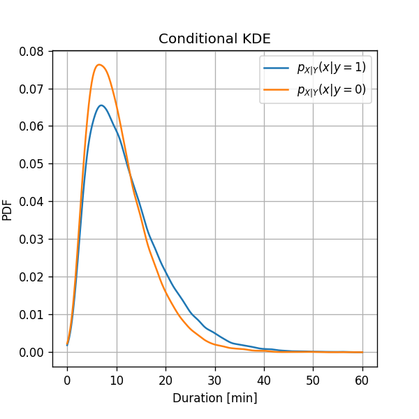
We can see here that during the work hours, $Y=1$, a ride has a slightly higher probability to have a longer duration. Let us see if we can use this fact to improve our prediction.

Solution Attempt 2: Prediction Based on Duration

Let us now try to improve our prediction using the duration data.

We would now like to make our prediction based on the the known duration of the ride:

I.e., we would like to predict: $\hat{y}\left(x\right)=\underset{y\in\left\lbrace 0,1\right\rbrace}{\arg\max}\ \ p_{Y|X}\left(y|x\right)$

• Given the input data $x$ of the specific ride, what is it $y$
• Instead of predicting the same value $\hat y$ for all the rides, we predict a prediction function $\hat y(x)$

Which is equivalent to: $\hat{y}\left(x\right) =\underset{y\in\left\lbrace 0,1\right\rbrace}{\arg\max}\ \ p_{Y|X}\left(y|x\right) = \begin{cases} 1 & p_{Y|X}\left(y=1|x\right)\geq p_{X|Y}\left(y=0|x\right) \\ 0 & \text{otherwise} \end{cases}$

We can will use Bayes rule:

$$p_{Y|X}\left(y|x\right)=\frac{p_{X|Y}\left(x|y\right)\cdot p_Y\left(y\right)}{p_X\left(x\right)}$$

To evaluate the condition in the prediction function:

$$p_{Y|X}\left(1|x\right)\overset{?}{\geq}p_{Y|X}\left(0|x\right) \\ \Leftrightarrow \frac{p_{X|Y}\left(x|1\right)\cdot p_Y\left(1\right)}{p_X\left(x\right)}\overset{?}{\geq}\frac{p_{X|Y}\left(x|0\right)\cdot p_Y\left(0\right)}{p_X\left(x\right)} \\ \Leftrightarrow p_{X|Y}\left(x|1\right)\cdot p_Y\left(1\right)\overset{?}{\geq}p_{X|Y}\left(x|0\right)\cdot p_Y\left(0\right)$$

Since we have a method for calculating $p_Y\left(y\right)$ and $p_{X\lvert Y}\left(x\lvert y\right)$ we can evaluate the above inequality for any given $x$. Let us calculate the prediction over a grid of durations:

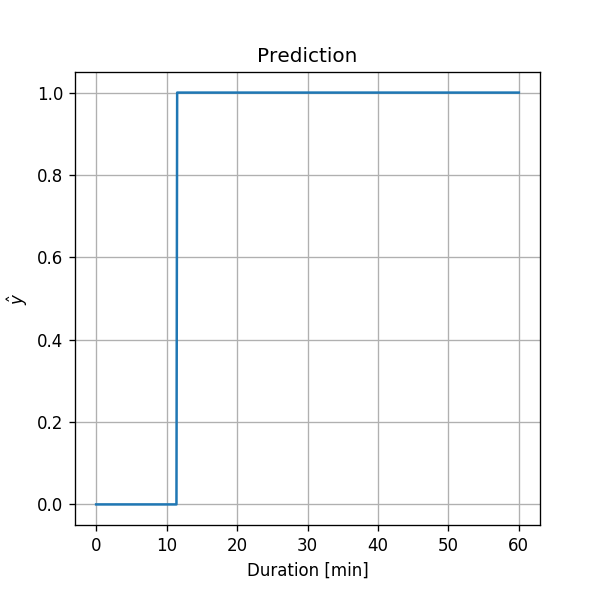
Therefore our prediction would be:

$$\hat{y}\left(x\right)= \begin{cases} 1 & x\geq11.4 \\ 0 & \text{otherwise} \end{cases}$$

⏱️ Performance evaluation - Based on Duration

Let us test our full prediction method on the test set:

The test risk is: $R_\text{test}\{ \hat{y}(x) \}=0.46$

We were able to slightly improve our prediction by using the ride duration.

As we add more data fields such as the length of the ride, the location, etc., we will be able to further improve our prediction.