Workshop 12

AdaBoost

AdaBoost (Adaptive Boosting) is a technique for improving the performance of a given classification algorithm by taking a smart weighted sum of multiple instances of the classifier.

This technique is based on iteratively building the series of classifier while keeping a vector of weights of how good was each point classified by previous classifiers. In each step the algorithm tries to build a classifier which corrects the errors made by previous classifiers.

Using the following notation:

$N$ - Is the size of the dataset
$\left\lbrace\boldsymbol{x}_i,y_i\right\rbrace$ - Are the measurements and the labels.
The labels $\left\lbrace y_i\right\rbrace$ have $1,-1$ values.

the steps of this algorithm are as follow:

Initialize a uniform weights vector for each data points: $w^{\left(t=0\right)}_i=\frac{1}{N}$
Iterate over the following steps, with a index , until reaching some stopping criteria:
1. Build an optimal classifier $h_t$ according to the given weighted dataest.
2. Calculate the prediction error of $h_t$ on the weighted dataset: $\varepsilon=\sum_i w^t_iI\left\lbrace h\left(\boldsymbol{x}_i\right)\neq y_i\right\rbrace$
3. Calculate the the weight for the $h_t$ classifier according to: $\alpha_t=\frac{1}{2}\ln\left(\frac{1-\varepsilon}{\varepsilon}\right)$
4. Update the weights of the data according to $w^t_i=w^{t-1}_i\exp\left(-\alpha_ty_ih_t\left(\boldsymbol{x}_i\right)\right)$
5. Normalize the weight by $Z=\sum_iw^t_i$ according to: $w^t_i=\frac{w^t_i}{Z}$

The final prediction will then be the following linear combination of the trained classifiers: $h\left(\boldsymbol{x}_i\right)=\text{sign}\left(\sum_t\alpha_th_t\left(\boldsymbol{x}_i\right)\right)$

Workshop 12
AdaBoost

Problem: Back to the Titanic

We will return to the problem from workshop 1 of trying to predict whether a passenger on board the Titanic has survived or not based on the data from the passengers manifest.

Dataset: The Titanic Manifest

The full manifest data can be found here with some additional details regarding the dataset.

A cleaner version of it for our needs can be found here.

🔃 The Workflow

We will follow the usual work follow to build our digits classifier

🛠️ Preparations

# Importing packages
import numpy as np  # Numerical package (mainly multi-dimensional arrays and linear algebra)
import pandas as pd  # A package for working with data frames
import matplotlib.pyplot as plt  # A plotting package

## Setup matplotlib to output figures into the notebook
## - To make the figures interactive (zoomable, tooltip, etc.) use ""%matplotlib notebook" instead
%matplotlib inline

plt.rcParams['figure.figsize'] = (5.0, 5.0)  # Set default plot's sizes
plt.rcParams['figure.dpi'] =120  # Set default plot's dpi (increase fonts' size)
plt.rcParams['axes.grid'] = True  # Show grid by default in figures

## A function to add Latex (equations) to output which works also in Google Colabrtroy
## In a regular notebook this could simply be replaced with "display(Markdown(x))"
from IPython.display import HTML
def print_math(x):  # Define a function to preview markdown outputs as HTML using mathjax
    display(HTML(''.join(['<p><script src=\'https://cdnjs.cloudflare.com/ajax/libs/mathjax/2.7.3/latest.js?config=TeX-AMS_CHTML\'></script>',x,'</p>'])))

🕵️ Data Inspection

Like always, we will start by loading the data and taking a look at it by printing out the 10 first rows.

data_file = 'https://yairomer.github.io/ml_course/datasets/titanic_manifest.csv'

## Loading the data
dataset = pd.read_csv(data_file)

## Print the number of rows in the data set
number_of_rows = len(dataset)
print_math('Number of rows in the dataset: $$N={}$$'.format(number_of_rows))

## Show the first 10 rows
dataset.head(10)

Number of rows in the dataset: $N=1001$

	pclass	survived	name	sex	age	sibsp	parch	ticket	fare	cabin	embarked	boat	body	home.dest	numeric_sex
0	1	1	Allen, Miss. Elisabeth Walton	female	29	0	0	24160	211.3375	B5	S	2	NaN	St Louis, MO	1
1	1	0	Allison, Miss. Helen Loraine	female	2	1	2	113781	151.5500	C22 C26	S	NaN	NaN	Montreal, PQ / Chesterville, ON	1
2	1	0	Allison, Mr. Hudson Joshua Creighton	male	30	1	2	113781	151.5500	C22 C26	S	NaN	135.0	Montreal, PQ / Chesterville, ON	0
3	1	0	Allison, Mrs. Hudson J C (Bessie Waldo Daniels)	female	25	1	2	113781	151.5500	C22 C26	S	NaN	NaN	Montreal, PQ / Chesterville, ON	1
4	1	1	Anderson, Mr. Harry	male	48	0	0	19952	26.5500	E12	S	3	NaN	New York, NY	0
5	1	1	Andrews, Miss. Kornelia Theodosia	female	63	1	0	13502	77.9583	D7	S	10	NaN	Hudson, NY	1
6	1	0	Andrews, Mr. Thomas Jr	male	39	0	0	112050	0.0000	A36	S	NaN	NaN	Belfast, NI	0
7	1	1	Appleton, Mrs. Edward Dale (Charlotte Lamson)	female	53	2	0	11769	51.4792	C101	S	D	NaN	Bayside, Queens, NY	1
8	1	0	Artagaveytia, Mr. Ramon	male	71	0	0	PC 17609	49.5042	NaN	C	NaN	22.0	Montevideo, Uruguay	0
9	1	0	Astor, Col. John Jacob	male	47	1	0	PC 17757	227.5250	C62 C64	C	NaN	124.0	New York, NY	0

The Data Fields and Types

In this workshop we will use the following fields:

pclass: the ticket’s class: 1st, 2nd or 3rd: 1, 2 or 3
sex: the sex of the passenger as a string: male or female
age: the passenger’s age: an integer
sibsp: the number of Siblings/Spouses aboard for each passenger: an integer
parch: the number of Parents/Children aboard for each passenger: an integer
fare: The price the passenger payed for the ticket: a positive real number
embarked: The port in which the passenger embarked the ship: (C = Cherbourg; Q = Queenstown; S = Southampton)
survived: The label for whether or not this passenger has survived: 0 or 1

(A full description for each of the other columns can be found here)

📉 Some Plots

Let us plot the survival of passengers as a function of each of the features.

discrete_columns = ['pclass', 'sex', 'sibsp', 'parch', 'embarked']
continuous_columns = ['age', 'fare']

## Plotting the histograms
fig, ax_list = plt.subplots(2, 4, figsize=(10, 5))
for i, feature in enumerate(discrete_columns):
    ax = ax_list.flat[i]
    dataset.groupby([feature, 'survived']).size().unstack('survived').plot.bar(ax=ax, stacked=True, legend=False)
    ax.set_title(feature)

for i, feature in enumerate(continuous_columns):
    ax = ax_list.flat[i + len(discrete_columns)]
    ax.hist(dataset.query('survived == 0')[feature].values, bins=20, alpha=0.5, label='0')
    ax.hist(dataset.query('survived == 1')[feature].values, bins=20, alpha=0.5, label='1')
    ax.set_title(feature)
    
for ax_list2 in ax_list:
    ax_list2[0].set_ylabel('Number of passengers')
    
ax_list.flat[-2].legend()
plt.tight_layout()

png

To make the dataset more useful to work with we will change all the discrete features to be numeric and start at 0 (we will treat sibsp and parch as finite discrete features):

dataset2 = pd.DataFrame({
    'survived': dataset['survived'],
    'pclass': dataset['pclass'].map({1:0, 2:1, 3:2}),
    'sex': dataset['sex'].map({'male':0, 'female':1}),
    'sibsp': dataset['sibsp'],
    'parch': dataset['parch'],
    'embarked': dataset['embarked'].map({'C':0, 'Q':1, 'S':2}),
    'age': dataset['age'],
    'fare': dataset['fare'],
    })

dataset2.dropna(axis=0, inplace=True)
dataset2['embarked'] = dataset2['embarked'].astype(int)
dataset2['weights'] = np.ones(len(dataset2)) / len(dataset2)

📜 Problem Definition

For the following given random system:

Random sample: $\omega$ - A passenger on board the Titanic.
Random variables:
- $\boldsymbol{x}=X\left(\omega\right)$ : The passenger parameters extracted from the manifest.
- $y=Y\left(\omega\right)$ : An indicator of whether or not the passenger survived.

Find a binary discrimination function $\hat{y}=h^*\left(\boldsymbol{x}\right)$ which minimizes the misclassification rate:

$h^*=\underset{h}{\arg\min}\ E\left[I\left\lbrace h\left(\boldsymbol{x}\right)\neq y\right\rbrace\right]$

💡 Model & Learning Method Suggestion: Stumps + AdaBoost

We will use Stumps classifiers (one level decision trees) which are boosted using AdaBoost.

We will use the weighted Gini index to build our classifiers using the weighted data. For a given split of the data in to $\mathcal{C}_1$ and $\mathcal{C}_2$ and a set of weights $\left\lbrace w_i\right\rbrace$ , the weighted Gini index will be:

$N_1=\sum_{i\in\mathcal{C}_1}w_i\\ N_2=\sum_{i\in\mathcal{C}_2}w_i\\ p_1=\frac{1}{N_1}\sum_{i\in\mathcal{C}_1}w_iI\left\lbrace y_i=1\right\rbrace\\ p_2=\frac{1}{N_2}\sum_{i\in\mathcal{C}_2}w_iI\left\lbrace y_i=1\right\rbrace\\ G=N_1p_1\left(1-p_1\right)+N_2p_2\left(1-p_2\right)$

Parameters:

The splitting performed by each stump.
The weighting of the stumps. $\alpha_i$ .

Hyper-parameters

The only parameter in this case is the stopping criteria of the the AdaBoost algorithm which defines the number of Stumps.

Data preprocessing

📚 Splitting the dataset

We will split the dataset into 80% train - 20% test.

n_samples = len(dataset2)

## Generate a random generator with a fixed seed
rand_gen = np.random.RandomState(0)

## Generating a vector of indices
indices = np.arange(n_samples)

## Shuffle the indices
rand_gen.shuffle(indices)

## Split the indices into 80% train / 20% test
n_samples_train = int(n_samples * 0.8)
n_samples_test = n_samples - n_samples_train
train_indices = indices[:n_samples_train]
test_indices = indices[n_samples_train:]

train_set = dataset2.iloc[train_indices]
test_set = dataset2.iloc[test_indices]

⚙️ Learning

Implementing a single stump

def calc_gini_on_split(split, y, weights):
    """
    A function for calculating the the weighted Gini index for a given split of the data.
    """
    
    ## Handle the case of a degenerated split
    if np.count_nonzero(split) == 0 or np.count_nonzero(split) == len(split):
        return np.inf
    
    ## The ratio of positive labels in branch 1
    p1 = (split * y * weights).sum() / (split * weights).sum()
    ## The ratio of positive labels in branch 2
    p2 = ((1 - split) * y * weights).sum() / ((1 - split) * weights).sum()
    ## The Gini index
    res = p1 * (1 - p1) * (split * weights).sum() + p2 * (1 - p2) * ((1 - split) * weights).sum()
    return res

class Stump:
    """
    A class for fitting and predicting a single stump
    """
    def __init__(self):
        self.split_mask = None
        self.threshold = None
        self.field = None
    
    def fit(self, dataset, field):

        self.field = field
        self.is_discrete = field in ['pclass', 'sex', 'sibsp', 'parch', 'embarked']
        
        ## Extrac relevat data for the dataset
        x = dataset[self.field].values
        y = dataset['survived'].values
        weights = dataset['weights'].values
        n_unique_vals = len(np.unique(x))
        
        if self.is_discrete:
            ## The finit discrete case
            ## A trick for generating all possible splits
            tmp = np.arange(2 ** n_unique_vals, dtype=np.uint8)
            all_possibles_splits = np.unpackbits(tmp[:, None], axis=1)[1:-1, -n_unique_vals:].astype(int)
            
            ## Loop over possible splits to look for the optimal split
            gini_min = np.inf
            for split_mask in all_possibles_splits:
                cls = split_mask[x]
                gini = calc_gini_on_split(cls, y, weights)
                if gini < gini_min:
                    gini_min = gini
                    self.split_mask = split_mask
        
        else:
            ## The continues case
            
            ## Al relevant thresholds
            all_possibles_thresholds = (x[:-1] + x[1:]) / 2
            
            ## Looping over thresholds
            gini_min = np.inf
            for threshold in all_possibles_thresholds:
                cls = x > threshold
                gini = calc_gini_on_split(cls, y, weights)
                if gini < gini_min:
                    gini_min = gini
                    self.threshold = threshold
        
        self.gini = gini_min
        
        return self
    
    def predict(self, dataset):
        x = dataset[self.field].values
        if self.is_discrete:
            y = self.split_mask[x]
        else:
            y = x > self.threshold
        
        return y
    
    def print_stump(self):
        if self.is_discrete:
            print('Classifing {} according to: {}'.format(self.field,
                                                          {0: np.where(1 - self.split_mask)[0].tolist(),
                                                           1: np.where(self.split_mask)[0].tolist()}))
        else:
            print('Classifing according to: {} > {}'.format(self.field, self.threshold))

Implementing AdaBoost

class AdaBoost:
    """
    A class which implaments the AdaBoost algorithm
    """
    def __init__(self, dataset):
        self.dataset = dataset.copy()
        self.y = self.dataset['survived'].values
        self.stumps_list = []
        self.alpha_list = []
        
        self.dataset['weights'] = np.ones(len(self.dataset)) / len(self.dataset)
    
    def fit_step(self, field):
        stump = Stump().fit(self.dataset, field)
        y_hat = stump.predict(self.dataset)
        err = (self.dataset['weights'].values * (self.y != y_hat)).sum()
        alpha = 0.5 * np.log((1 - err) / err)
        self.dataset['weights'] *= np.exp(-alpha * ((self.y == y_hat) * 2 - 1))
        self.dataset['weights'] /= self.dataset['weights'].sum()
        self.stumps_list.append(stump)
        self.alpha_list.append(alpha)

        print('Error: {}'.format(err))
        print('Alpha: {}'.format(alpha))
        stump.print_stump()
        
    def plot(self):
        discrete_columns = ['pclass', 'sex', 'sibsp', 'parch', 'embarked']
        continuous_columns = ['age', 'fare']

        ## Plotting the histograms
        fig, ax_list = plt.subplots(2, 4, figsize=(10, 5))
        for i, feature in enumerate(discrete_columns):
            stump = Stump().fit(self.dataset, feature)
            ax = ax_list.flat[i]
            self.dataset.groupby([feature, 'survived'])['weights'].sum().unstack('survived')\
                                                        .plot.bar(ax=ax, stacked=True, legend=False)
            ax.set_title('{}\n{:.3f}'.format(feature, stump.gini))

        for i, feature in enumerate(continuous_columns):
            stump = Stump().fit(self.dataset, feature)
            ax = ax_list.flat[i + len(discrete_columns)]
            ax.hist(self.dataset.query('survived == 0')[feature].values, 
                    weights=self.dataset.query('survived == 0')['weights'].values,
                    bins=20, alpha=0.5, label='0')
            ax.hist(self.dataset.query('survived == 1')[feature].values,
                    weights=self.dataset.query('survived == 1')['weights'].values,
                    bins=20, alpha=0.5, label='1')
            ax.set_title('{}\n{:.3f}'.format(feature, stump.gini))

        for ax_list2 in ax_list:
            ax_list2[0].set_ylabel('Number of passengers')

        ax_list.flat[-2].legend()
        plt.tight_layout()
    
    def predict(self, dataset):
        y_hat = np.zeros(len(dataset))
        for alpha, stump in zip(self.alpha_list, self.stumps_list):
            y_hat += alpha * (stump.predict(dataset) * 2 - 1)
        y_hat = y_hat > 0
        return y_hat

Training

Initializing the Algorithm

adaboost = AdaBoost(train_set)

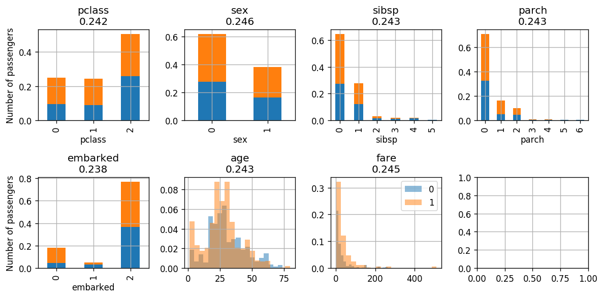
Let us print the data weights and plot the distributions according to the weighted data:

adaboost.plot()
adaboost.dataset.head(10)

	age	embarked	fare	parch	pclass	sex	sibsp	survived	weights
724	11	2	46.9000	2	2	0	5	0	0.001252
77	27	2	30.5000	0	0	0	0	1	0.001252
879	6	2	21.0750	1	2	0	3	0	0.001252
615	22	2	7.2500	0	2	0	1	0	0.001252
905	24	2	8.6625	0	2	0	0	0	0.001252
533	42	2	7.5500	0	2	0	0	0	0.001252
401	50	2	13.0000	0	1	0	0	0	0.001252
454	39	2	26.0000	0	1	0	0	0	0.001252
31	58	2	26.5500	0	0	1	0	1	0.001252
358	18	2	13.0000	0	1	0	0	0	0.001252

png

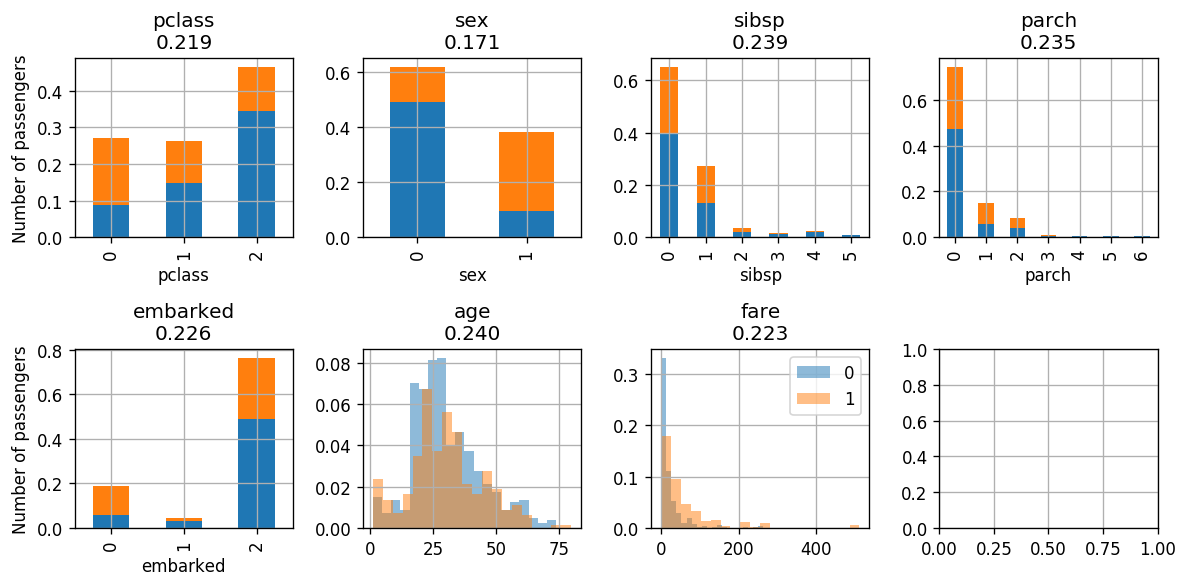
The Weighted Gini Indexes are plotted in the title. In each step we will select the feature with the lowest index. In this case this will be the sex.

Iteration: $t=1$

Classiffing according to the sex

adaboost.fit_step('sex')
adaboost.plot()
adaboost.dataset.head(10)

Error: 0.22027534418022526
Alpha: 0.6320312618746508
Classifing sex according to: {0: [0], 1: [1]}

	age	embarked	fare	parch	pclass	sex	sibsp	survived	weights
724	11	2	46.9000	2	2	0	5	0	0.000803
77	27	2	30.5000	0	0	0	0	1	0.002841
879	6	2	21.0750	1	2	0	3	0	0.000803
615	22	2	7.2500	0	2	0	1	0	0.000803
905	24	2	8.6625	0	2	0	0	0	0.000803
533	42	2	7.5500	0	2	0	0	0	0.000803
401	50	2	13.0000	0	1	0	0	0	0.000803
454	39	2	26.0000	0	1	0	0	0	0.000803
31	58	2	26.5500	0	0	1	0	1	0.000803
358	18	2	13.0000	0	1	0	0	0	0.000803

png

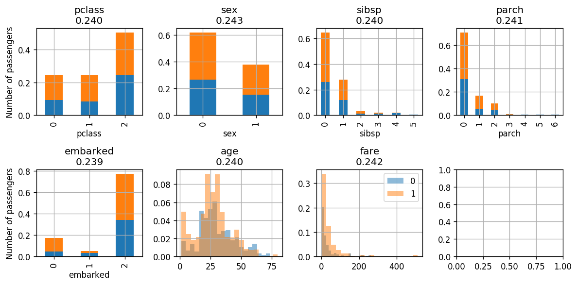
We will see that as we advance through the algorithm the weighted data becomes more uniformly distributed as a function of the labels, i.e. the distributions of the data with $y=1$ will be as the same as the distribution of the data with $y=-1$ .

As a consequences of that, the classification task will become harder and the classifier’s classification error will go to 0.5.

In addition the weighting parameter $\alpha_t$ will decrease over time.

Next we will classify according to the pclass which has the lowest index.

Iteration $T=2$

adaboost.fit_step('pclass')
adaboost.plot()
adaboost.dataset.head(10)

Error: 0.6677960382314314
Alpha: -0.3491168359813891
Classifing pclass according to: {0: [0], 1: [1, 2]}

	age	embarked	fare	parch	pclass	sex	sibsp	survived	weights
724	11	2	46.9000	2	2	0	5	0	0.000601
77	27	2	30.5000	0	0	0	0	1	0.002127
879	6	2	21.0750	1	2	0	3	0	0.000601
615	22	2	7.2500	0	2	0	1	0	0.000601
905	24	2	8.6625	0	2	0	0	0	0.000601
533	42	2	7.5500	0	2	0	0	0	0.000601
401	50	2	13.0000	0	1	0	0	0	0.000601
454	39	2	26.0000	0	1	0	0	0	0.000601
31	58	2	26.5500	0	0	1	0	1	0.000601
358	18	2	13.0000	0	1	0	0	0	0.000601

png

Next we will classify according to the embarked which has the lowest index.

Iteration $T=3$

adaboost.fit_step('embarked')
adaboost.plot()
adaboost.dataset.head(10)

Error: 0.5323984758056922
Alpha: -0.06488786721923188
Classifing embarked according to: {0: [0], 1: [1, 2]}

	age	embarked	fare	parch	pclass	sex	sibsp	survived	weights
724	11	2	46.9000	2	2	0	5	0	0.000564
77	27	2	30.5000	0	0	0	0	1	0.002274
879	6	2	21.0750	1	2	0	3	0	0.000564
615	22	2	7.2500	0	2	0	1	0	0.000564
905	24	2	8.6625	0	2	0	0	0	0.000564
533	42	2	7.5500	0	2	0	0	0	0.000564
401	50	2	13.0000	0	1	0	0	0	0.000564
454	39	2	26.0000	0	1	0	0	0	0.000564
31	58	2	26.5500	0	0	1	0	1	0.000643
358	18	2	13.0000	0	1	0	0	0	0.000564

png

adaboost.fit_step('embarked')
adaboost.plot()
adaboost.dataset.head(10)

Error: 0.5000000000000001
Alpha: -2.2204460492503136e-16
Classifing embarked according to: {0: [0], 1: [1, 2]}

	age	embarked	fare	parch	pclass	sex	sibsp	survived	weights
724	11	2	46.9000	2	2	0	5	0	0.000564
77	27	2	30.5000	0	0	0	0	1	0.002274
879	6	2	21.0750	1	2	0	3	0	0.000564
615	22	2	7.2500	0	2	0	1	0	0.000564
905	24	2	8.6625	0	2	0	0	0	0.000564
533	42	2	7.5500	0	2	0	0	0	0.000564
401	50	2	13.0000	0	1	0	0	0	0.000564
454	39	2	26.0000	0	1	0	0	0	0.000564
31	58	2	26.5500	0	0	1	0	1	0.000643
358	18	2	13.0000	0	1	0	0	0	0.000564

png

We eventually reached a point where the classifier’s classification error is very close to 0.5 and $alpha_t$ is very small.

⏱️ Performance evaluation

Let us calculate the risk on the test set

x_train = train_set[discrete_columns + continuous_columns].values
y_train = train_set['survived'].values

x_test = test_set[discrete_columns + continuous_columns].values
y_test = test_set['survived'].values

predictions = adaboost.predict(test_set)
# predictions = adaboost.stumps_list[0].predict(test_set)

test_risk = (y_test != predictions).mean()
print_math('The test risk is: $${:.3}$$'.format(test_risk))

The test risk is: $0.225$

%%html
<link rel="stylesheet" href="../css/style.css"> <!--Setting styles - You can simply ignore this line-->

Workshop 12

AdaBoost

AdaBoost

Workshop 12AdaBoost

Problem: Back to the Titanic

Dataset: The Titanic Manifest

🔃 The Workflow

🛠️ Preparations

🕵️ Data Inspection

The Data Fields and Types

📉 Some Plots

📜 Problem Definition

💡 Model & Learning Method Suggestion: Stumps + AdaBoost

Parameters:

Hyper-parameters

Data preprocessing

📚 Splitting the dataset

⚙️ Learning

Implementing a single stump

Implementing AdaBoost

Training

Initializing the Algorithm

Iteration: t=1

Iteration T=2

Iteration T=3

⏱️ Performance evaluation

Workshop 12
AdaBoost

Iteration: $t=1$

Iteration $T=2$

Iteration $T=3$