Workshop 01 Introduction

Goals

These workshops come to accompany the lectures and recitations by taking another dive into the subjects of this course, but from a more "hands-on" approach. The purpose of the workshops is to achieve the following goals:

The primary goal: Improve the understanding and intuition behind the methods taught in the course by applying them to examples, and discussing the different nuances of each method.

The secondary goal: Provide tools for approaching and solving machine learning real problems in real life by using state of the art tools to problem sets which are based on real data.

Relation to Homework Assignment¶

The hands-on part ("wet" part) of the homework assignment will be of the same form of implementation section of the workshops.

A comment about the code¶

In many cases, the code and algorithms in these workshops are written in a very inefficient way. We have preferred to keep the code readable and as close as possible to the algorithm described in class. In almost all cases, there already exist packages implementing these algorithms efficiently and robustly, when possible we have tried to give references to these implementations.

This Workshop

In this workshop, we will mainly be discussing the process which we will be using for solving the problem. The rest of the workshops will mainly discuss the different approaches and methods which we can use when applying this process.

Why ?

Here are some motivational points for why we decided on teaching using Python, and why should you learn it?

It is a very powerful programing language and yet very simple to learn and to get started with. (See what XKCD has to say about it)
It is currently one of the most popular programming languages. (It is the 3rd most popular language, after C and Java, according to this survey)
Almost all new frameworks in the field of machine learning are developed for python: PyTorch, TensorFlow, Keras, etc.
It has a ridiculously rich set of packages for almost any task. From basic mathematical tools(basic numeric, advance numerics, symbolic math data handling, visualizing, etc.), through a range of advanced frameworks for deep learning, distributed computing, web servers, etc. and up to stuff such as a complete framework for writing simple games
It's open-source (=> free) with a huge community behind it.

Jumping Into The Water

We will start by jumping directly into the water by applying a simple solution to a popular introductory problem

At this point, we will do it in a very sloppy way, and the solution we will get will be very far from idle. The goal here is only to build the overall idea of the type of problems we will be trying to solve and the general process we are going to apply for solving them.

We will later come back to this exact problem again and solve it using some more advanced tools while defining everything in a much more formal way.

The Titanic Prediction Problem

In this problem, we would like to predict whether or not a given passenger has survived the Titanic tragedy based only the passengers' details in manifest which contains some cold facts such as age, sex, the ticket class, etc.

To be able to come up with a good prediction method we are given a portion of the passenger manifest along with the data of whether or not these passengers have survived. The goal would be to be able to provide a good prediction for the survival chances for passengers outside this list.

Here are some reasons to believe why we might be able to improve our guess based on these cold facts are:

Mid-age people might be better swimmers then very young or old people, therefore their chances for survival might be higher.
The different classes on board the Titanic were located in different areas of the boat, so maybe they were affected differently by the impact with the iceberg.
It might be that most of the people on board the Titanic were in fact proper gentlemen and gave the women priority when boarding the lifeboats.
etc.

The workflow

Throughout the workshops, we will try to build and follow a certain workflow which we will apply to the problems we come to solve. For now, we will only give a general description of the process, and as we advance we will gain a better understanding and obtain more tools for applying in each of the steps. We will start with the following diagram and make some small adaptations to it as we advance in the course:

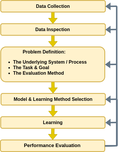
This course we will mostly focus on the two steps of suggesting a model and a learning method and applying them.

Let us try to understand this workflow by applying it to the problem at hand. For now, we will only give a very general description of each step, in a future workshop, we will provide a more in-depth descriptions for each of the steps.

Applying the Workflow¶

We will start by importing some useful packages

## Importing packages
import numpy as np  # Numerical package (mainly multi-dimensional arrays and linear algebra)
import pandas as pd  # A package for working with data frames
import matplotlib.pyplot as plt  # A plotting package

%matplotlib inline

## A function to add Latex (equations) to output which works also in Google Colabrtroy
## In a regular notebook this could simply be replaced with "display(Markdown(x))"
from IPython.display import HTML
def print_math(x):  # Define a function to preview markdown outputs as HTML using mathjax
    display(HTML(''.join(['<p><script type="text/x-mathjax-config">MathJax.Hub.Config({tex2jax: {inlineMath: [[\'$\',\'$\'], [\'\\\\(\',\'\\\\)\']]}});</script><script src=\'https://cdnjs.cloudflare.com/ajax/libs/mathjax/2.7.3/latest.js?config=TeX-AMS_CHTML\'></script>',x,'</p>'])))

Data collection

In our problem, we will only work with pre-collected datasets, and won't discuss this step at all. It is, however, vital to understand that this step is an integral part of the process and in many cases will be evolving over time to better fit the needs of the system.

Data Inspection

Let us take a look at the dataset. In many cases, such as this one, it is convenient to store the data as a table (or a matrix) where:

Each column represents one of the collected data fields. In our case: age, gender, ticket class, etc.
Each row represents a single observation. In our case a single passenger. Each observation is called a sample.

We will start by loading the data and taking a look at it by printing out the 10 first rows.

The data can be found at https://technion046195.github.io/semester_2019_spring/datasets/titanic_manifest.csv

data_file = 'https://technion046195.github.io/semester_2019_spring/datasets/titanic_manifest.csv'

## Loading the data
dataset = pd.read_csv(data_file)

## Print the number of rows in the data set
number_of_rows = len(dataset)
print_math('Number of rows in the dataset: $N={}$'.format(number_of_rows))

## Show the first 10 rows
dataset.head(10)

The Data Fields and Types¶

For simplicity, in this exercise will limit ourselves to using only these three fields:

numerical_sex: the sex of the passenger as a number: 0 - male, 1 - female (a boolean).
pclass: the ticket's class: 1st, 2nd or 3rd (a class indicator).
survived: Whether or not this passenger has survived (a boolean)

(A full description for each of the other columns can be found here)

Problem Definition

The Underlying Process¶

In this step, we will define the process which generates the data, usually in a probabilistic manner. For now, we will choose to describe the process as some back box which randomly spits out pairs of some passenger parameters and an indicator of whether this passenger has survived or not. An important assumption we make on the process is that different outcomes are statistically independent.

This process of randomly generating passengers and survival outcome can be thought of as the random chain of events which lead certain passengers to board the Titanic and the event which eventually resulted in whether or not they have survived.

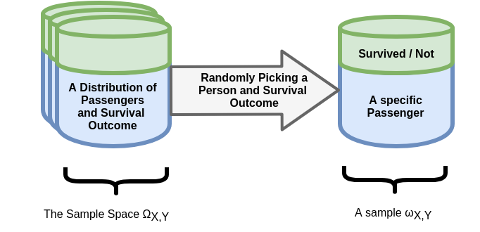
We assume that the dataset was generate by apply this process $N$ times, with $N$ being the size of the dataset.

The Task and the Goal\n",¶

As stated before, in this problem we would like to come up with a method, for guessing, or predicting whether or not a passenger on board the Titanic has survived the crash based on his properties.

i.e., we are looking for a function which maps from the input space of gender and class, $\boldsymbol{x}$, into the binary space of the survival indicator, $y$:

$$ \hat{y}=h\left(\boldsymbol{x}\right) $$

Where we have defined $\hat{y}$ as our prediction for the input $\boldsymbol{x}$.

We will later in this course define these type of problems as binary classification problems.

Evaluation Method: The Misclassification Rate¶

We still have not formally define what we mean by making a good prediction. In order to be able to pick the best prediction function, we must first define a way to evaluate different functions.

We would usually want to be able to assign a numeric score of how bad a prediction function performs and then strive to pick the function with the lowest score. We would call this function the risk function.

In this case, we will use a risk function called the misclassification rate. The misclassification rate is defined as the prediction errors a function makes on the data. Denoting:

$N$ - the number of sample in the dataset.
$\boldsymbol{x}_i$ - the person parameters in the $i$'s sample, i.e., the vector of $\left(\text{gender},\text{class}\right)$ of the $i$'s passenger.
$I\left\{\text{condition}\right\}$- an indicator function returning 1 if the condition is true and 0 otherwise

The risk would be:

$$ R\left\{h, \left\{\boldsymbol{x},y\right\}\right\}=\frac{1}{N}\sum_i I\left\{h\left(\boldsymbol{x}_i\right)\neq y_i\right\} $$

A comment about naming: In many places, this function appears under different names. Other common names for this function are the cost function, the error function or the loss function.

Although the name loss function is very commonly used, especially in deep learning, in our course, we will stick to the name risk and have a different definition for the term of a loss function.

Splitting the dataset¶

We will be using our dataset for two different tasks:

Producing the prediction function.
Evaluating the performance.

This is a bit problematic, since in general, this will result in an optimistic result. The fact that our solution performs well on the given data does not necessarily mean that it will perform well on any new data.

A Simple Example¶

Let us suppose that the names of the passengers are part of the input data. In this case, we could propose a prediction method which memorizes the list of surviving passengers and makes a prediction based on that list. This method will perform great on the given data, but it would fail for any new data.

A simple solution is to leave a portion of the dataset for the use of evaluation only. These two portions of the dataset are usually referred to as the train set and the test set.

A common practice is to use an 80% train-20% test split. In most cases, it will be important to split the data randomly independently of the order of the sample in the original dataset.

Let us prepare our dataset and split it to the train set and test set.

## Preparing the data set
## Constructing x_{i,j} and y_i. Here i runs over the passengers and j runs over [gender, class]
x = dataset[['numeric_sex', 'pclass']]
y = dataset['survived']

n_samples = len(x)

## Generate a random generator with a fixed seed (this is important to make our result reproducible)
rand_gen = np.random.RandomState(0)

## Generating a vector of indices
indices = np.arange(n_samples)

## Shuffle the indices
rand_gen.shuffle(indices)

## Split the indices into 80% train / 20% test
n_samples_train = int(n_samples * 0.8)
n_samples_test = n_samples - n_samples_train
train_indices = indices[:n_samples_train]
test_indices = indices[n_samples_train:]

## Split the data
x_train = x.iloc[train_indices]
x_test = x.iloc[test_indices]
y_train = y.iloc[train_indices]
y_test = y.iloc[test_indices]

## We could have directly shuffled and split the data, but in this way, we are still left with the original data and the indices which were used for the split which could be useful, especially for debugging.

Model & Learning Method Suggestion

In this step, we would like to suggest a family of optional solutions for our problem. We would then have to search the space of suggested solutions to select the best solution according to our evaluation method. I.e., we would search for the solution which produces in the minimal risk. We should note here that in many cases, finding the solution with the lowest risk is not possible and we would settle for the solution with the lowest risk we can find.

These solutions families will usually, but not always, be defined by a set of parameters. In such cases, we will use $\theta$ to denote these parameters.

We refer to this family of solutions as the model.

There are many consideration which come into account for selecting different models. We will point out three of them:

It should be a model for which we have an efficient method for finding the solution with the lowest risk.
It should be a model which cover an extensive range of solutions in order to increase our chance of coming up with a solution which produces a low risk.
As we will see, in many cases if the range of solution is too wide we will usually encounter a problem called overfitting, therefore in some cases we would not want the range of solutions to be too extensive. We will elaborate much more on this subject later in this course.

In our example we will suggest a model for the prediction function $h\left(\boldsymbol{x}\right)$. In fact in this simple example, since $h\left(\boldsymbol{x}\right)$ has only 6 possible inputs (2 gender x 3 classes), we can use 6 binary parameters to define the whole set of possible functions $h\left(\boldsymbol{x}\right)$.

$$ h_\boldsymbol{\theta}\left(\boldsymbol{x}\right)=\left\{ \begin{array}{ll} \theta_{0, 1} & \boldsymbol{x}=\left(0, 1\right) \\ \theta_{0, 2} & \boldsymbol{x}=\left(0, 2\right) \\ \theta_{0, 3} & \boldsymbol{x}=\left(0, 3\right) \\ \theta_{1, 1} & \boldsymbol{x}=\left(1, 1\right) \\ \theta_{1, 2} & \boldsymbol{x}=\left(1, 2\right) \\ \theta_{1, 3} & \boldsymbol{x}=\left(1, 3\right) \\ \end{array} \right. $$

reminder: $\boldsymbol{x}=\left(\text{gender}, \text{class}\right)$

As a more visually appealing way, we can also write it in the form of a table:

Sex \ Class	1st class	2nd Class	3rd class
Male (0)	$\theta_{0,1}$	$\theta_{0,2}$	$\theta_{0,3}$
Female (1)	$\theta_{1,1}$	$\theta_{1,2}$	$\theta_{1,3}$

Only for demonstrating the process, we will start with an even more simplified model for $h_\boldsymbol{\theta}\left(\boldsymbol{x}\right)$. We will start with the family of constant functions, i.e., $h_\theta\left(\boldsymbol{x}\right)=\theta$

Sex \ Class	1st class	2nd Class	3rd class
Male (0)	$\theta$	$\theta$	$\theta$
Female (1)	$\theta$	$\theta$	$\theta$

Our method for finding the constant function, or equivalently the $\theta$, which produces the lowest risk would be to test all possible options. Since we are talking about a binary prediction function, there are only 2 options: $h_{\theta=0}\left(\boldsymbol{x}\right)=0$ and $h_{\theta=1}\left(\boldsymbol{x}\right)=1$,

Learning

Here we will usually apply some fancy method for selecting the best method, in this case, we simply need to evaluate the risk for the two options of $\theta=0$ and $\theta=1$ and one which produces the lower result.

Formally we would like to find the optimal value of $\theta$, which we will denote as $\theta^*$, for which:

$$ \theta^* =\underset{\theta\in\left\{0,1\right\}}{\arg\min}\ R\left\{h_{\theta}, \left\{\boldsymbol{x} ,y\right\}\right\} =\underset{\theta\in\left\{0,1\right\}}{\arg\min}\ \frac{1}{N}\sum_i I\left\{\theta\neq y_i\right\} $$

Let us calculate the risk for each $\theta$ (note that we will only be using the train set for this task) :

## Loop over the two possible theta
print('The train risk for each predictor is:')
for theta in [0, 1]:
    ## The number of worng prediction for theta:
    predictions = theta
    train_risk = (y_train.values != predictions).mean()
    print_math('- $R_\\text{{train}}\\{{ h_{{ \\theta={} }} \\}}={:.2}$'.format(theta, train_risk))

The train risk for each predictor is:

In this case, constantly predicting zero performs slightly better than constantly predicting one.

This is due to the fact that the majority of passengers did not survive the crash, therefore without knowing any details about the passenger we have a better change predicting that he did not survive.

Our proposed prediction function would be: $$ h\left(\boldsymbol{x}\right)=0\quad\forall\boldsymbol{x} $$

Performance Evaluation

As stated before would like to do the evaluating of the risk on the test set. Let us calculate the risk using the test set.

## The evaluation of the final risk
predictions = 0
test_risk = (y_test.values != predictions).mean()
print_math('The test risk is: $R_\\text{{test}}\\{{ h_{{ \\theta=0 }} \\}}={:.2}$'.format(test_risk))

We would now want to suggest a way to improve our learning method.

In this case, the obvious way to get improvement is by replacing the naive model which we have used. Let us go back to the model suggestion stage.

Model & Learning Method Suggestion - 2nd Attempt

Let us now return to the full model for $h_\boldsymbol{\theta}\left(\boldsymbol{x}\right)$ which covers all the possible all possible $2^6$ combinations for selecting $\boldsymbol{\theta}=\left(\theta_{0,1},..,\theta_{1,3}\right)^T$.

It could be shown that in this case, that we can find the optimal selection of the $\theta_{m,n}$'s by looking at each one of them individually and minimize the risk on the group of passengers with $X=\left(m,n\right)$. I.e.

$$ \theta_{m,n}^* =\underset{\theta_{m,n}\in\left\{0,1\right\}}{\arg\min}\ R\left\{h_{\boldsymbol{\theta}}, \left\{\boldsymbol{x}_i ,y_i:\boldsymbol{x}_i=\left(m,n\right)\right\}\right\} =\underset{\theta_{m,n}\in\left\{0,1\right\}}{\arg\min}\ \frac{1}{N_{m,n}}\sum_{i,\boldsymbol{x}_i=\left(m,n\right)} I\left\{\theta_{m,n}\neq y_i\right\} $$

with $m\in\left\{0,1\right\}$ (the gender) and $n\in\left\{1,2,3\right\}$ (the class)

print('The train risk for each group is:')
## loop over the gender
for gender in [0, 1]:
    ## loop over the class
    for class_ in [1, 2, 3]:  # we have used "class_" since the word "class" is already in use by python
        print('')  # An empty line
        print_math('## For $\\{{\\boldsymbol{{x}}_i,y_i:\\boldsymbol{{x}}_i=({},{}) \\}}$'.format(gender, class_))
        ## Loop over the two possible theta
        for theta in [0, 1]:
            ## The number of worng prediction for theta:
            predictions = theta
            indices = (x_train['numeric_sex'].values == gender) & (x_train['pclass'].values == class_)
            train_risk = (y_train.values[indices] != predictions).mean()
            print_math('-- $\\theta_{{ {},{} }}={} \Rightarrow R_{{\\text{{train}}}}\\{{h_{{ \\boldsymbol{{\\theta}} }}\\}}={:.2f}$'.format(gender, class_, theta, train_risk))

The train risk for each group is:

Therefore our optimal predictor $\boldsymbol{\theta}^*$ will be constructed by choosing for each $\theta_{m,n}$ the values which minimizes the risk:

Sex \ Class	1st class	2nd Class	3rd class
Male (0)	0	0	0
Female (1)	1	1	0

Performance Evaluation

Let us calculate the risk for this prediction function

## The optimal predictor

## We will define a prediction function which recives a row in the 
## dataset as an input and outputs a predition
def row_predictor(row):
    gender = row['numeric_sex']
    class_ = row['pclass']
    
    prediction_map = {
        (0, 1): 0,
        (0, 2): 0,
        (0, 3): 0,
        (1, 1): 1,
        (1, 2): 1,
        (1, 3): 0,
    }
    
    prediction = prediction_map[(gender, class_)]
    return prediction

## Apllying the predicion function to every line in the table
predictions = x_test.apply(row_predictor, axis='columns')

## The evaluation of the final risk
test_risk = (y_test.values != predictions).mean()
print_math('The test risk is: $R_\\text{{test}}\\{{ h_{{ \\boldsymbol{{\\theta}}^* }} \\}}={:.2f}$'.format(test_risk))

This mean that by using this predictor we have will be able to give a correct prediction about 77% of the time.

Conclusion

We have seen how we can use a dataset to build a model which we can now be used to make predictions on data we have not seen yet. We did so following a general workflow which we have described.

In almost all of the problems which we will solve in these workshops, we will follow this workflow. The parts which will change from one problem/solution to another is:

The problem, goal and evaluation method.
The part of the system which we will be modeling.
The set of models we will be using in the model suggestion step.
The learning method which we will be using for selecting a good model from within the set of models.
Some additional variations of the learning method, which deal with a problem called overfitting.

Attributions

Icons in these notebooks were made by:

https://icons8.com is licensed by CC 3.0 BY-ND
Freepik from https://www.flaticon.com is licensed by CC 3.0 BY

%%html
<link rel="stylesheet" href="../css/style.css"> <!--Setting styles - You can simply ignore this line-->

	pclass	survived	name	sex	age	sibsp	parch	ticket	fare	cabin	embarked	boat	body	home.dest	numeric_sex
0	1	1	Allen, Miss. Elisabeth Walton	female	29	0	0	24160	211.3375	B5	S	2	NaN	St Louis, MO	1
1	1	0	Allison, Miss. Helen Loraine	female	2	1	2	113781	151.5500	C22 C26	S	NaN	NaN	Montreal, PQ / Chesterville, ON	1
2	1	0	Allison, Mr. Hudson Joshua Creighton	male	30	1	2	113781	151.5500	C22 C26	S	NaN	135.0	Montreal, PQ / Chesterville, ON	0
3	1	0	Allison, Mrs. Hudson J C (Bessie Waldo Daniels)	female	25	1	2	113781	151.5500	C22 C26	S	NaN	NaN	Montreal, PQ / Chesterville, ON	1
4	1	1	Anderson, Mr. Harry	male	48	0	0	19952	26.5500	E12	S	3	NaN	New York, NY	0
5	1	1	Andrews, Miss. Kornelia Theodosia	female	63	1	0	13502	77.9583	D7	S	10	NaN	Hudson, NY	1
6	1	0	Andrews, Mr. Thomas Jr	male	39	0	0	112050	0.0000	A36	S	NaN	NaN	Belfast, NI	0
7	1	1	Appleton, Mrs. Edward Dale (Charlotte Lamson)	female	53	2	0	11769	51.4792	C101	S	D	NaN	Bayside, Queens, NY	1
8	1	0	Artagaveytia, Mr. Ramon	male	71	0	0	PC 17609	49.5042	NaN	C	NaN	22.0	Montevideo, Uruguay	0
9	1	0	Astor, Col. John Jacob	male	47	1	0	PC 17757	227.5250	C62 C64	C	NaN	124.0	New York, NY	0